2 Methods
2.1 Site description
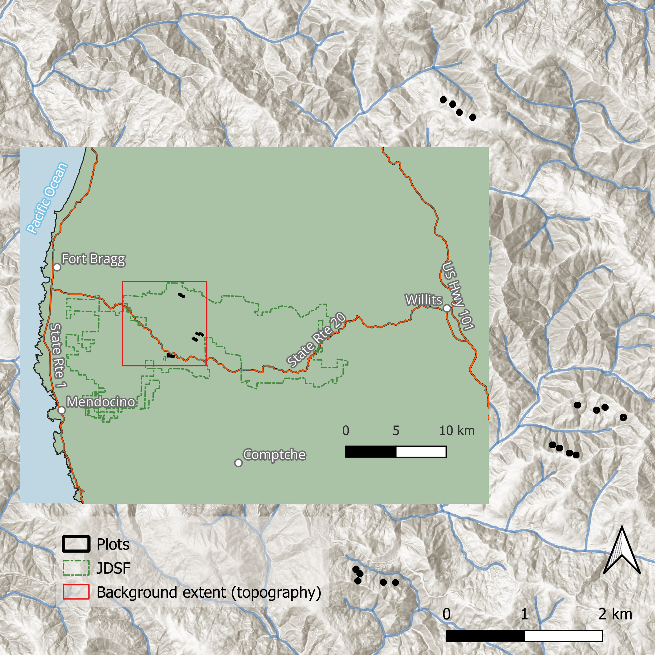
Situated within the unceded ancestral territory of the Northern Pomo, near the coast of Northern California, the 20,000-ha Jackson Demonstration State Forest (JDSF) was established in 1947 after being cut over multiple times starting in 1862. The mission of the JDSF is to remain in timber production for research and demonstration purposes. The predominant cover type is redwood, tanoak, and Douglas-fir forest at elevations ranging from 20 m near the coast to 700 m inland. The climate is Mediterranean with cool, wet winters and an average annual precipitation of about 1150 mm. The sites that compose our experiment were all redwood dominated with significant components of tanoak and Douglas-fir and were well stocked with trees 80 to 100 years old. All of our study sites are between 13 and 16 km from the Pacific Ocean at elevations between 130 and 300 m, on well-drained, sandstone-derived soils. The sites are located on various aspects on mid to upper-slope positions (Figure 2.1), and the site quality is classified as Site Class II (Lindquist & Palley, 1963; Webb et al., 2012).
2.2 Study design
In 2012, four treatments were replicated at four different sites. The treatments were: group selection (GS), high-density dispersed retention (HD), high-density aggregated retention (HA), and low-density dispersed retention (LD). The GS treatment is composed of a circular 1-ha opening in which all trees were removed, surrounded by a 50-meter buffer of light thinning in which less than 1/3 of the basal area was removed. The remaining treatments were applied over 2-hectare treatment units. The target post-harvest density was specified in terms of relative density using an assumed upper stand density index (SDI) limit for redwood of 2,470 stems ha-1 (Reineke, 1933). The target residual relative density for the HA and HD treatments was 21% (SDI = 520), and the for the LD treatment it was 13% (SDI = 320). These densities were chosen to balance the objectives of stand volume production and individual tree growth assuming a subsequent, similar harvest after 20 years (Berrill & O’Hara, 2009).
After harvesting, a single 0.2-hectare square macro plot was established in the center of each treatment unit. Approximately 25 redwood and 25 tanoak sprout clumps that were well distributed across the plot, were selected for measurement. Additionally, for redwood, sprout clumps were selected evenly from those with, and without residual standing trees.
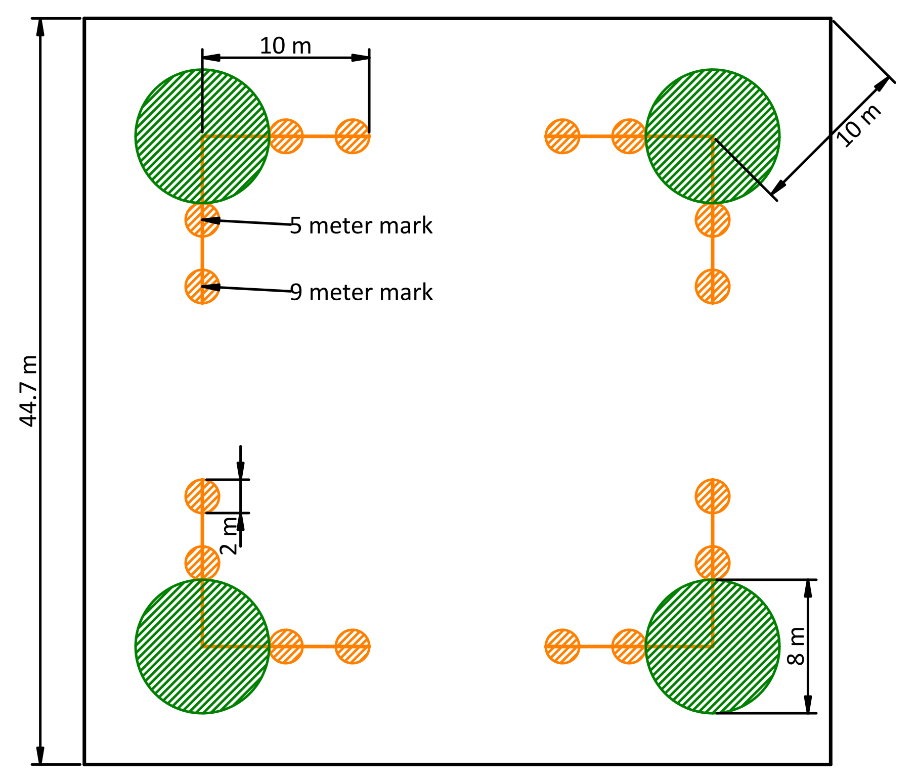
Ten years after the initial harvest, regeneration plots and fuel transects were established within the macro plot (Figure 2.2). Circular regeneration plots with a 4-meter radius were established 10 meters from each macro plot corner, towards the plot center. Terminating at the center of each of these regeneration plots, 10-meter fuel transects were established parallel to the macro plot edges. Live fuels were estimated in 1-meter radius “sampling cylinders” at the five-, and nine-meter locations along each transect.
Following year 10 measurements, all plots received a PCT treatment where the objective was to release merchantable conifers such as redwood and Douglas-fir from competition. Competing trees and shrubs were cut, lopped, and scattered within the measurement plots and fuel transects were re-measured.
2.3 Data collection
2.3.1 Regeneration
Ten years after the initial harvest, four four-meter-radius regeneration plots were established within each macro plot (Figure 2.2). All regenerating trees (sprouts and seedlings) within the plot were recorded. Regenerating trees less than 5 cm diameter at breast height (1.4 m) were tallied by 2.5 cm size classes and the actual DBH of all other regenerating trees were recorded. This allowed for an estimation of sprout and seedling density by species.
2.3.2 Sprout size
Sprout height data were collected during the winter at years 1, 5, and 10 following the initial harvest. Sprout heights at each period were based on the tallest individual within the selected redwood and tanoak clumps at the time of measurement with a height pole placed at the same location on the ground at each measurement period. The observer eliminated parallax by observing from a location up-slope, level with the height of the sprout. Sprout DBH for only redwood was collected in year 10.
2.3.3 Fuels
Also at 10 years after the initial harvest, fuel transects were established and sampled according to the FIREMON protocol (Lutes et al., 2006), with some adaptations that were unique to this project. This protocol is very similar to that of Brown (1974). One-, 10-, 100-hr, and 1000-hr (or coarse woody) fuels were those less than 0.635 cm, 0.635 to 2.54 cm, 2.54 to 7.62 cm and those 7.62 cm and greater, respectively and included only dead and downed woody fuels (not those attached to live vegetation, or standing dead). Transect lengths for 1-, 10-, and 100-hr fuels were two, two, and four meters, respectively during pre-PCT measurements. During post-PCT measurement, the length of the 1-hr fuel transect was reduced to one meter because of the dramatic increase in these fuels. Coarse woody fuels were measured along the entire 10-meter transect.
Redwoods, like other species in Cupressaceae, shed branchlets instead of individual leaves. This leads to difficulty in distinguishing “litter” from 1-hr fuels. We chose to use an estimated cutoff of about 2 mm for redwood branchlets, where larger pieces were considered 1-hr fuel and smaller pieces were considered part of the litter layer. We did not distinguish between “leafy” and “awl like” leaf shapes (Graham, 2009).
Live vegetation percent cover and average height were estimated in 1-meter-radius “sampling cylinders” as described in the FIREMON protocol (Lutes et al., 2006). A notable exception is that the sampling cylinders were allowed to extend to the (average) top height of the live fuels that were continuous within less than a meter of the ground. This resulted in average live vegetation heights that could sometimes reach near the height of the sprouts and average heights above two meters were estimated with the help of a clinometer. This decision makes explicit instances when when fuels are vertically continuous with the ground. Live vegetation percent cover was estimated for four vegetation classes: live woody fuels, dead woody fuels, live herbaceous fuels, and dead herbaceous fuels. Dead “live” fuels includes dead fuels attached to live plants, or those still rooted in the ground. Particles in these conditions are not counted as downed woody fuels when tallying fine and coarse woody fuels along fuel transects. These fuels are, though, expected to behave differently during combustion than live “live” fuels. Average vegetation height was recorded for two classes: the average height of all woody fuels and the average height of all herbaceous fuels. These estimates pertain to the particles present in the sampling cylinder, and not the area-average, thus a cylinder with only one percent cover, could still have an average height of two meters, i.e., the empty space within the cylinder does not affect the average height. The average height and percent-cover estimates are visual estimations and efforts were made to compare these frequently to ensure that estimates among observers were consistent. Percent cover estimates were discrete, rounded to the nearest class in the set: 0.5, 3, 10, and all subsequent 10 percent increments up to 100 percent.
The depth of duff and litter was measured at one representative location within each of the two, 1-meter-radius sampling cylinders along each transect. When duff and litter conditions varied greatly in a single sampling cylinder, a location was chosen to represent the average of conditions within the cylinder.
Fuel bed depth was estimated as the average height of the fine and coarse woody debris components within each sampling cylinder. Theoretically, this included litter, but not duff. This estimate was not described in the FIREMON protocol, but it was designed to be made in a similar manner as described for vegetation heights.
2.4 Analysis
An analysis was conducted in three stages, one for each of the three response categories: fuels, sprout size, and regeneration density. All analyses were conducted using R and attempts were made to document all data, decisions, and techniques within a Quarto notebook, which is published at https://fisher-j.github.io/multi-age. All response variables were analyzed using multi-level models to account for the inherent nesting structure of the data, including multiple measurements of sprouts over time, where applicable. Grouping levels were included in the models if their variance estimate was determined to be significant. If including a grouping level resulted in a meaningful change in estimates or confidence intervals, the grouping level was kept. Because the overall objective was to detect differences between treatments, treatment was used as the primary independent variable. Model development and selection were carried out using Akaike information criterion, Bayesian information criterion, and visualization of (probability integral) transformed residuals (Hartig, 2022). Models were built using the R package GLMMtmb, which provides a consistent framework for exploring different response distributions and link functions as well as the ability to model variance as a function of predictors (Brooks et al., 2017). The final model structures chosen for each response are given in the results section.
Models were interpreted using estimated marginal means calculated with the R packages marginaleffects and emmeans (Arel-Bundock et al., 2024; Lenth, 2021). Predictions incorporating the effects of all model components were made on the response scale for a grid of predictors consisting of all unique combinations of factors in the data that were used in at least one component of a given model (we didn’t have numeric predictors) except in the case of tree heights where predictions were made for each observation in the data set. Standard errors for the predictions were calculated using the delta method. Predictions were averaged across non-focal predictors (especially “random” effects) to obtain the population estimates of marginal means. These means are expected to be applicable to other treatments when conducted across equal proportions of sites with conditions similar to those used in our study. Notably, our population estimates assume equal proportions of north and south facing aspects.
2.4.1 Regeneration
Sprout count data from our 4-meter-radius regeneration plots were converted to basal area per acre per species. Tallies of species by size class for sprouts less than 5 cm dbh were converted to diameters using the class midpoint (1.27 or 3.81 cm) before calculating basal area per acre. Minor species (i.e., those other than redwood, tanoak, and Douglas-fir) were combined into an “other” category. Missing species on a plot were made explicit by assigning a value of 0 m2 ha-1 for that species and plot. In addition to basal area, Douglas-fir stem counts (stems ha-1) were modeled separately.
2.4.2 Sprout heights
Two metrics were analyzed from the sprout height data: height increment (m year-1), and total height (m) at year 10. For height increment, there were two measurements for each tree: increment for years 1 to 5 and increment for years 5 to 10. Thus, analysis of these data included tree as a candidate random effect. While not making a difference for analysis results, it is worth noting that these data were structured differently from the other datasets in that plot was made a globally unique identifier, thus making explicit the nesting of plots within sites or treatments and eliminating the need to specify this nesting structure in the R code model formulas.
2.4.3 Fuels
Fuel load in Mg ha-1 was estimated for 1-hr, 10-hr, 100-hr, combined duff and litter (“duff/litter”), 1,000-hr, and live vegetation fuels at the transect level. Any transect where a fuel type was not observed was assigned a value of zero for that class and transect. Fuel load for 1- through 1,000-hr fuels were calculated using the method in Brown (1974). The required size-class specific parameters (specific gravity, particle inclination, and average diameter) were derived from a previous study where I used parameters averaged across all of the measured plots (Glebocki, 2015). For 1,000-hr fuels, decay classes 1-3 were considered “sound” and decay classes 4 and 5 were considered “rotten” for the purpose of calculating load and these loads were combined. Duff and litter were measured at two locations along each transect and these were averaged at the transect level. We did not measure the bulk density of duff and litter fuels, but based on findings in other studies in the redwood region, we opted to combine these classes into a single fuel class, using an average bulk density found across those studies of 7.73 Mg ha-1 (Finney & Martin, 1993; Kittredge, 1940; Stuart, 1985). Vegetation fuel load was calculated using bulk density constants of 8 Mg ha-1 m-1 for herbaceous fuels and 18 Mg ha-1 m-1 for woody components (Gangi, 2006). Live and dead components were combined to calculate herbaceous and woody loading. Herbaceous and woody fuel loads were then combined and averaged at the transect level (two measurements per transect) to determine total vegetation loading.