Family: Gamma (log)
Conditional: ba_ha ~ treat * spp + (1 | site:spp)
Dispersion: ~spp (log)
Hurdle: ~spp (logit) 3 Results
The formulas below use \(\beta\) to represent fixed effects and \(\alpha\) to represent random effects. Subscripts indicate the variable associated with each effect. Superscripted Greek letters indicate the model component where fixed or random effects are present in more than one component (e.g., \(\mu\) for the conditional model, \(\pi\) for the hurdle model, and \(\phi\) for the dispersion model). A “hurdle gamma” distribution is used for models of basal area and fuels and is defined below.
\[ \text{hurdle\_gamma}(y_i \mid \pi_i, \mu_i, \phi_i) = \begin{cases} 1-\pi_i & \text{if } y_i = 0 \\ \pi_i \cdot \text{Gamma}(y_i \mid \mu_i, \phi_i) & \text{if } y_i > 0 \end{cases} \]
3.1 Regeneration
3.1.1 Basal area
Composition of regeneration in terms of basal area per acre represented by each species in a 4-meter radius vegetation plot was modeled as a gamma distribution with a log link with fixed effects for treatment and species, and random intercepts for site x species interaction. Dispersion was modeled separately as a function of species, using a log link and the rate of zeros was modeled using the logit link, for each species as well:
\[ Y_i \sim \text{hurdle\_gamma}(\pi_i, \mu_i, \phi_i) \]
\[ \text{logit}(\pi_i) = \beta^{\pi}_0 + \beta^{\pi}_{\text{spp}} \cdot \text{Species}_i \]
\[ \log(\mu_i) = \beta^{\mu}_0 + \beta^{\mu}_{\text{trt}} \cdot \text{Trt} + \alpha_{j[i]} \]
\[ \log(\phi_i) = \beta^{\phi}_0 + \beta^{\phi}_{\text{spp}} \cdot \text{Species}_i \]
\[ \alpha_j \sim N(0, \sigma^2_j) \]
- \(Y_i\): Total basal area per hectare for each species in a 4-meter radius regeneration plot.
- \(\pi_i\): Probability that \(Y_i > 0\)
- \(\mu_i\): Mean of positive values.
- \(\phi_i\): Dispersion parameter for Gamma distribution
- \(\alpha_j\): Group effect pertaining to a site:species interaction
Focal species for this model included redwood, tanaok, Douglas-fir, and other species.
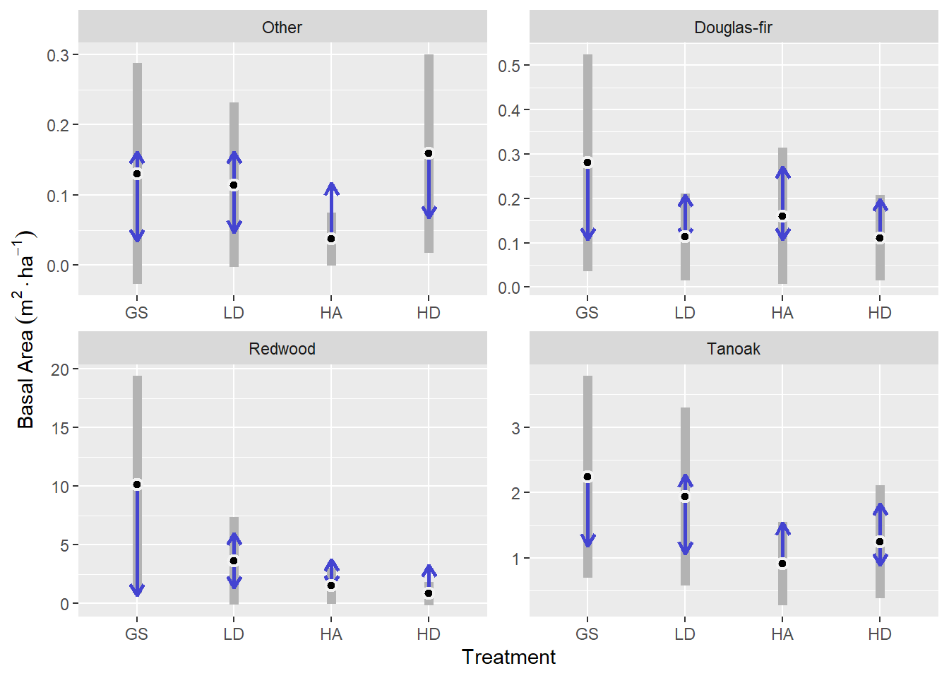
Redwood regeneration basal area showed the greatest treatment response. The GS treatment had the greatest basal area of redwood regeneration at 10.12 m2 ha-1, which was 9.28 m2 ha-1 greater than in the HD treatment (p = 0.19). The LD and HD treatments were intermediate.
Tanoak regeneration basal area was intermediate between that of redwood and Douglas-fir and other species. The GS and LD treatments had similar responses, as did the HA and HD treatments. The GS treatment resulted in 2.24 m2 ha-1 of tanoak basal area, which was 1.33 m2 ha-1 greater than in the HA treatment (p = 0.18).
On average, for Douglas-fir, we expect about 0.17 m2 ha-1 of basal area across treatments. The greatest basal area of Douglas-fir was in the GS treatment which was 0.12 m2 ha-1 greater than in the HA treatment (p = 0.76). The LD, HA, and HD treatments were all comparatively similar.
Other species included grand fir, madrone, and California wax-myrtle, of which there was a total of 23, 28, and 16 observations across our 16 macro plots (comprising 64 tree density plots). Generally, each plot had between 0 and 9 observations of other species, except for one macro plot with the LD treatment, which had 16 observations (data not shown).
According to predictions made from this model for other species, there was not enough evidence to confirm a statistically significant difference between treatments. On average, we expect about 0.11 m2 ha-1 of basal area across treatments. The greatest basal area of other species was in the HD treatment which was 0.12 m2 ha-1 greater than in the HA treatment (p = 0.26). The GS and LD treatments were intermediate.
| Spp | Emmean | SE | 95% LCL | 95% UCL |
|---|---|---|---|---|
| other | 0.11 | 0.04 | 0.03 | 0.19 |
| df | 0.17 | 0.06 | 0.05 | 0.28 |
| rw | 4.03 | 1.52 | 1.04 | 7.01 |
| to | 1.59 | 0.47 | 0.67 | 2.50 |
| Spp | treatment | Emmean | SE | 95% LCL | 95% UCL |
|---|---|---|---|---|---|
| other | gs | 0.13 | 0.08 | -0.03 | 0.29 |
| other | ld | 0.11 | 0.06 | -0 | 0.23 |
| other | ha | 0.04 | 0.02 | -0 | 0.07 |
| other | hd | 0.16 | 0.07 | 0.02 | 0.3 |
| df | gs | 0.28 | 0.12 | 0.04 | 0.52 |
| df | ld | 0.11 | 0.05 | 0.02 | 0.21 |
| df | ha | 0.16 | 0.08 | 0.01 | 0.31 |
| df | hd | 0.11 | 0.05 | 0.01 | 0.21 |
| rw | gs | 10.12 | 4.74 | 0.84 | 19.41 |
| rw | ld | 3.63 | 1.91 | -0.12 | 7.38 |
| rw | ha | 1.51 | 0.78 | -0.01 | 3.04 |
| rw | hd | 0.85 | 0.52 | -0.17 | 1.86 |
| to | gs | 2.24 | 0.79 | 0.7 | 3.79 |
| to | ld | 1.94 | 0.69 | 0.58 | 3.3 |
| to | ha | 0.92 | 0.33 | 0.28 | 1.56 |
| to | hd | 1.25 | 0.44 | 0.39 | 2.11 |
| Spp | Contrast | Emmean | SE | P value |
|---|---|---|---|---|
| other | gs - ld | 0.02 | 0.09 | 1 |
| other | gs - ha | 0.09 | 0.08 | 0.6 |
| other | gs - hd | -0.03 | 0.09 | 0.99 |
| other | ld - ha | 0.08 | 0.06 | 0.53 |
| other | ld - hd | -0.04 | 0.07 | 0.91 |
| other | ha - hd | -0.12 | 0.07 | 0.26 |
| df | gs - ld | 0.17 | 0.11 | 0.46 |
| df | gs - ha | 0.12 | 0.12 | 0.76 |
| df | gs - hd | 0.17 | 0.11 | 0.42 |
| df | ld - ha | -0.05 | 0.08 | 0.93 |
| df | ld - hd | 0 | 0.05 | 1 |
| df | ha - hd | 0.05 | 0.07 | 0.91 |
| rw | gs - ld | 6.49 | 4.6 | 0.49 |
| rw | gs - ha | 8.61 | 4.56 | 0.23 |
| rw | gs - hd | 9.28 | 4.64 | 0.19 |
| rw | ld - ha | 2.12 | 1.8 | 0.64 |
| rw | ld - hd | 2.79 | 1.83 | 0.42 |
| rw | ha - hd | 0.67 | 0.79 | 0.83 |
| to | gs - ld | 0.31 | 0.69 | 0.97 |
| to | gs - ha | 1.33 | 0.65 | 0.18 |
| to | gs - hd | 0.99 | 0.64 | 0.4 |
| to | ld - ha | 1.02 | 0.58 | 0.29 |
| to | ld - hd | 0.69 | 0.57 | 0.63 |
| to | ha - hd | -0.33 | 0.37 | 0.8 |
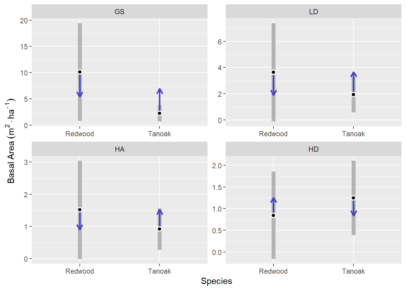
Figure 3.2 shows the same model as Figure 3.1, but with an emphasis on treatment comparisons between redwood and tanoak. This shows that we expect on average, 7.88 m2 ha-1 greater redwood basal area than tanoak basal area in the GS treatment (p = 0.1), about 1.69 m2 ha-1 in the LD treatment (p = 0.4), and about 0.6 m2 ha-1 in the HA treatment (p = 0.48). In the HD treatment, we expect to see slightly higher tanoak basal area (p = 0.55).
Uncertainty in average redwood basal area across sites, indicated by the size of 95% confidence intervals, is much greater than that of tanoak in the GS treatment, but this difference diminishes such that GS > LD > HA > HD (Figure 3.2). In the HD treatment redwood and tanoak average basal area uncertainty across sites is very similar.
3.1.2 Douglas-fir counts
Counts of regenerating Douglas-fir seedlings per vegetation plot were analyzed for differences between harvest treatments using a negative binomial response with a log link, fixed effects for treatment, random effects for sites and macro plots within sites.
Family: nbinom1 (log)
Conditional: n ~ treat + (1 | site) + (1 | site:treat)
\[ Y_i \sim \text{NB1}(\mu_i, \phi); \quad \text{where} \quad Var(Y_i) = \mu_i + \phi \mu_i \]
\[ \log(\mu_i) = \beta_0 + \beta_{\text{trt}} \cdot \text{Trt}_i + \alpha_{j[i]} + \alpha_{k[i]} \]
\[ \alpha_{j} \sim \operatorname{N}(0, \sigma^2_{j}), \quad \alpha_{k} \sim \operatorname{N}(0, \sigma^2_{k}) \]
- \(Y_i\): Count of Douglas-fir seedlings in a 4-meter radius vegetation plot.
- \(\mu_i\): The expected count for vegetation plot \(i\).
- \(\beta_{\text{trt}}\): Fixed effect for harvest treatment.
- \(\alpha_j\): Random intercept for site.
- \(\alpha_k\): Random intercept for plots within sites.
This model for Douglas-fir counts does not indicate any statistically significant differences between treatments. Generally, we expect about 2 seedlings per 4-meter-radius plot, or about 413 seedlings per hectare (Figure 3.3).
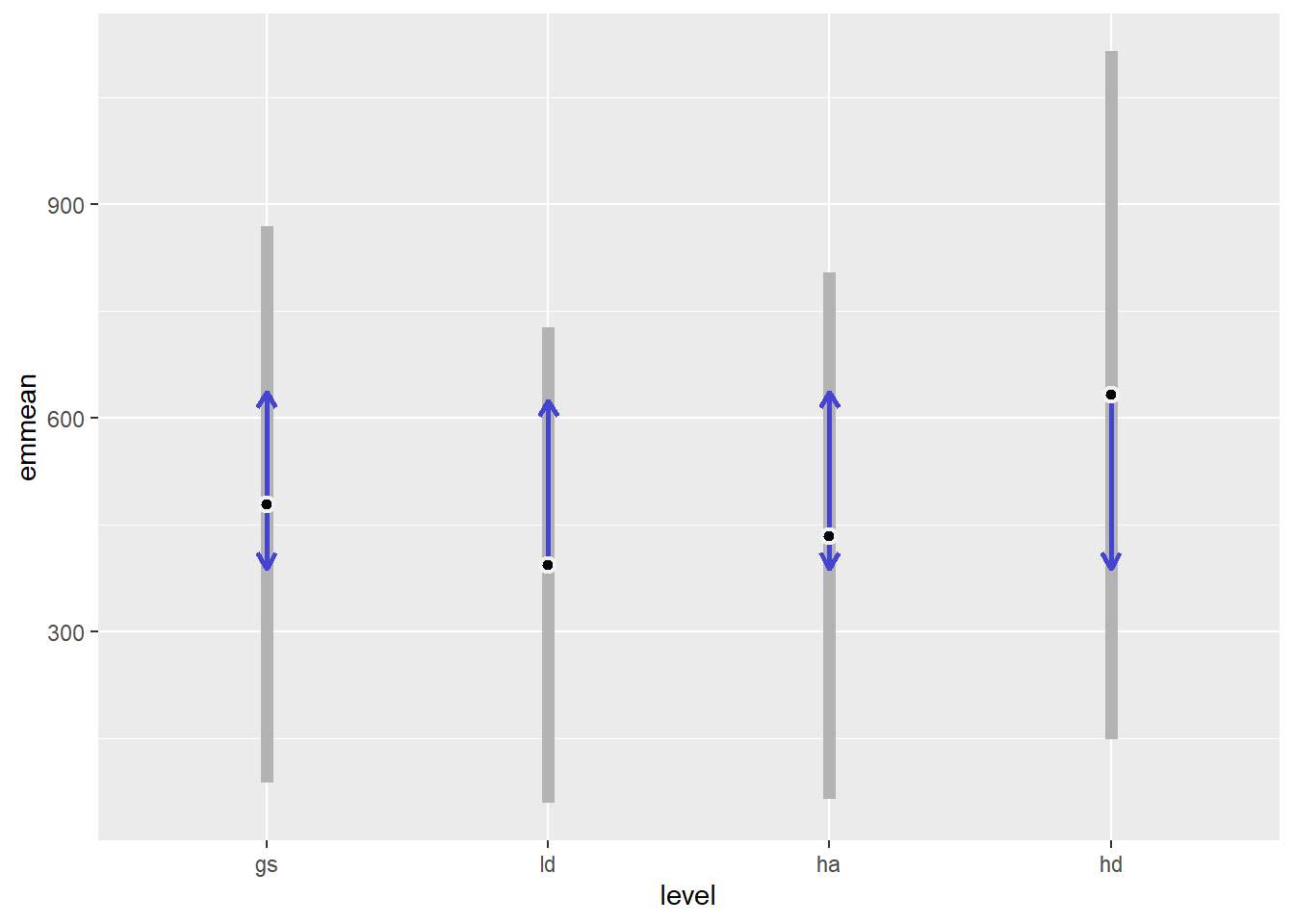
| Treatment | estimate | asymp.LCL | asymp.UCL |
|---|---|---|---|
| gs | 479 | 88 | 869 |
| ld | 394 | 60 | 728 |
| ha | 435 | 65 | 805 |
| hd | 632 | 149 | 1115 |
3.2 Sprout heights
In the following two models, a random slope for species is included for each macro plot. This specifies a general (unstructured) covariance matrix that allows the random effect variance to differ by species (heteroscedasticity) and allows for non-zero correlations between species-level effects within the same plot (e.g., assessing if plots that are favorable for one species are also favorable for others). This variance-covariance matrix takes the following form, where \(A\), \(B\), and \(C\) represent different species.
\[ \boldsymbol{\Sigma}_{\text{macro}} = \begin{pmatrix} \sigma_A^2 & \rho_{AB}\sigma_A\sigma_B & \rho_{AC}\sigma_A\sigma_C \\ \rho_{AB}\sigma_A\sigma_B & \sigma_B^2 & \rho_{BC}\sigma_B\sigma_C \\ \rho_{AC}\sigma_A\sigma_C & \rho_{BC}\sigma_B\sigma_C & \sigma_C^2 \end{pmatrix} \]
3.2.1 Height increment
The selected height increment model used a normal response distribution on the identity link. It included treatment, growth period, species, and the interaction of species and growth period as fixed effects. A random intercept was included for tree (multiple observations) and macro-plot, and another random effect allowed the response to vary by species differently for each macro plot. The dispersion parameter for the response was modeled (with a log link) as a function of treatment, growth period, species and all three-way interactions (Listing 3.3).
Family: gaussian (identity)
Conditional: ht_inc ~ treat + year * spp + (1 | tree) + (0 + spp | plot)
Dispersion: ~spp * year * treat (log)
\[ Y_i \sim \operatorname{N}(\mu_i, \sigma^2_i) \]
\[ \mu_i = \beta_0^{\mu} + \beta_{\text{trt}}^{\mu} \cdot \text{Trt}_i + \beta_{\text{year}}^{\mu} \cdot \text{Year}_i + \beta_{\text{spp}}^{\mu} \cdot \text{Spp}_i + \beta_{\text{spp:year}}^{\mu}(\text{Spp}_i \times \text{Year}_i) + \alpha_{\text{tree}[i]} + \alpha_{\text{macro}[i],\text{spp}[i]} \]
\[ \log(\sigma_i) = \beta^{\sigma}_0 + \beta^{\sigma}_{\text{trt}} \cdot \text{Trt}_i + \beta^{\sigma}_{\text{yr}} \cdot \text{Year}_i + \beta^{\sigma}_{\text{spp}} \cdot \text{Spp}_i + \dots + \beta^{\sigma}_{\text{3way}} (\text{Trt}_i \times \text{Year}_i \times \text{Spp}_i) \]
\[ \alpha_{\text{tree}} \sim N(0, \sigma^2_{\text{tree}}) \]
\[ \alpha_{\text{macro}, \text{spp}} = \begin{pmatrix} \alpha_{\text{macro}_1, \text{spp}_1} \\ \alpha_{\text{macro}_1, \text{spp}_2} \\ \vdots \\ \alpha_{\text{macro}_j, \text{spp}_k} \end{pmatrix} \sim \operatorname{N}(\mathbf{0}, \boldsymbol{\Sigma}_{\text{macro}}) \]
- \(Y_i\): Height increment (m yr-1) for sprout observation \(i\).
- \(\mu_i\): Mean height increment for observation \(i\).
- \(\sigma^2_i\): Variance of height increment for observation \(i\).
- \(\alpha^{\mu}_{\text{tree}}\): Random intercept for tree.
- \(\alpha^{\mu}_{\text{macro}, \text{spp}}\): Random effect for species, co-varying within macro plot.
- \(\boldsymbol{\Sigma}_{\text{macro}}\): Unstructured variance-covariance matrix for species within macro plot.
The model selected based on AIC lacks a treatment x species interaction, suggesting that there is not evidence that treatments affected species differentially. It also lacks a treatment x year interaction. This means that there was not enough evidence to support that treatment was related to changes in growth rate.
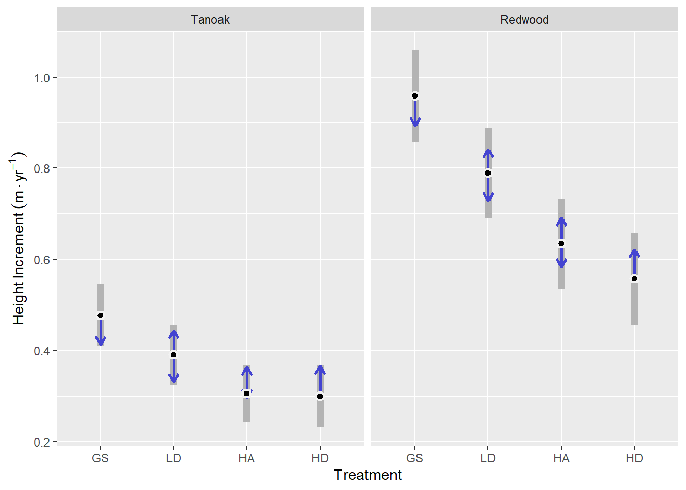
The inclusion of treatment factors in the model (0.001 ≤ p < 0.03) indicated that the levels of treatment were associated with different growth rates across species and years. And the species x year interaction (p < 0.001) suggested that changes in growth rates were different for redwood and tanoak (Figure 3.4).
For tanoak, height increment was greatest in the GS treatment at 0.48 m yr-1. This was about 0.17 m yr-1 more than in the HA and HD treatments, which were very similar at about 0.3 m yr-1.
Redwood followed a similar pattern but with more pronounced differences between treatments. Height increment for redwood in the GS treatment was 0.96 m yr-1, which was about 0.4 m yr-1 greater than in the HD treatment (p = 0). Additionally, there was evidence that the GS treatment led to greater height increment than the LD treatment by about 0.17 m yr-1 (p = 0). And the LD treatment was higher than the HA treatment by about 0.15 m yr-1 (p = 0).
| Spp | Treat | Emmean | SE | 95% LCL | 95% UCL |
|---|---|---|---|---|---|
| TO | GS | 0.48 | 0.034 | 0.41 | 0.54 |
| TO | LD | 0.39 | 0.033 | 0.32 | 0.46 |
| TO | HA | 0.31 | 0.032 | 0.24 | 0.37 |
| TO | HD | 0.3 | 0.034 | 0.23 | 0.37 |
| RW | GS | 0.96 | 0.052 | 0.86 | 1.06 |
| RW | LD | 0.79 | 0.051 | 0.69 | 0.89 |
| RW | HA | 0.63 | 0.05 | 0.54 | 0.73 |
| RW | HD | 0.56 | 0.052 | 0.46 | 0.66 |
Redwood growth slowed from 0.80 to 0.67 m yr-1 in the second period and tanoak slowed from 0.39 to 0.34 m yr-1.
Redwood grew faster than tanoak, but slowed down more relative to it in the second period. Height increment for redwood was 0.42 m yr-1 greater than tanoak in the first period and 0.33 m yr-1 greater than tanoak in the second period (Figure 3.5).

| Spp | Year | Emmean | SE | DF | 95% LCL | 95% UCL |
|---|---|---|---|---|---|---|
| TO | 5 | 0.39 | 0.017 | Inf | 0.35 | 0.42 |
| TO | 10 | 0.35 | 0.017 | Inf | 0.31 | 0.38 |
| RW | 5 | 0.8 | 0.043 | Inf | 0.72 | 0.89 |
| RW | 10 | 0.67 | 0.043 | Inf | 0.59 | 0.75 |
3.2.2 Height at year 10
Sprout heights at year 10 were modeled with a normal response and a log link. The best model included species and treatment, but no interactions in the fixed effects. This suggests that treatments do not affect species differentially in terms of the mean response (height at year 10). It also included a model for dispersion (log link) with predictors species, treatment, and their interaction (Listing 3.4).
Family: gaussian (log)
Conditional: ht ~ treat + spp + (0 + spp | plot)
Dispersion: ~spp * treat (log)
\[ Y_i \sim \operatorname{N}(\mu_i, \sigma^2_i) \]
\[ \log(\mu_i) = \beta_0^{\mu} + \beta_{\text{trt}}^{\mu} \cdot \text{Trt}_i + \beta_{\text{spp}}^{\mu} \cdot \text{Spp}_i + \alpha_{\text{spp}[i], \text{macro}[i]} \]
\[ \log(\sigma_i) = \beta^{\sigma}_0 + \beta^{\sigma}_{\text{trt}} \cdot \text{Trt}_i + \beta^{\sigma}_{\text{spp}} \cdot \text{Spp}_i + \beta^{\sigma}_{\text{trt:spp}}(\text{Trt}_i \times \text{Spp}_i) \]
\[ \alpha_{\text{spp}, \text{macro}} = \begin{pmatrix} \alpha_{\text{spp}_1, \text{macro}_1} \\ \alpha_{\text{spp}_1, \text{macro}_2} \\ \vdots \\ \alpha_{\text{spp}_j, \text{macro}_k} \end{pmatrix} \sim \operatorname{N}(\mathbf{0}, \boldsymbol{\Sigma}_{\text{spp}, \text{macro}}) \]
- \(Y_i\): Height at year 10 for tree \(i\).
- \(\mu_i\): Mean height at year 10 for tree \(i\).
- \(\sigma^2_i\): Variance of height at year 10 for tree \(i\).
- \(\alpha_{\text{macro}, \text{spp}}\): Random effect for species, co-varying within macro plot.
- \(\boldsymbol{\Sigma}_{\text{macro}, \text{spp}}\): Unstructured variance-covariance matrix for species within macro plot.
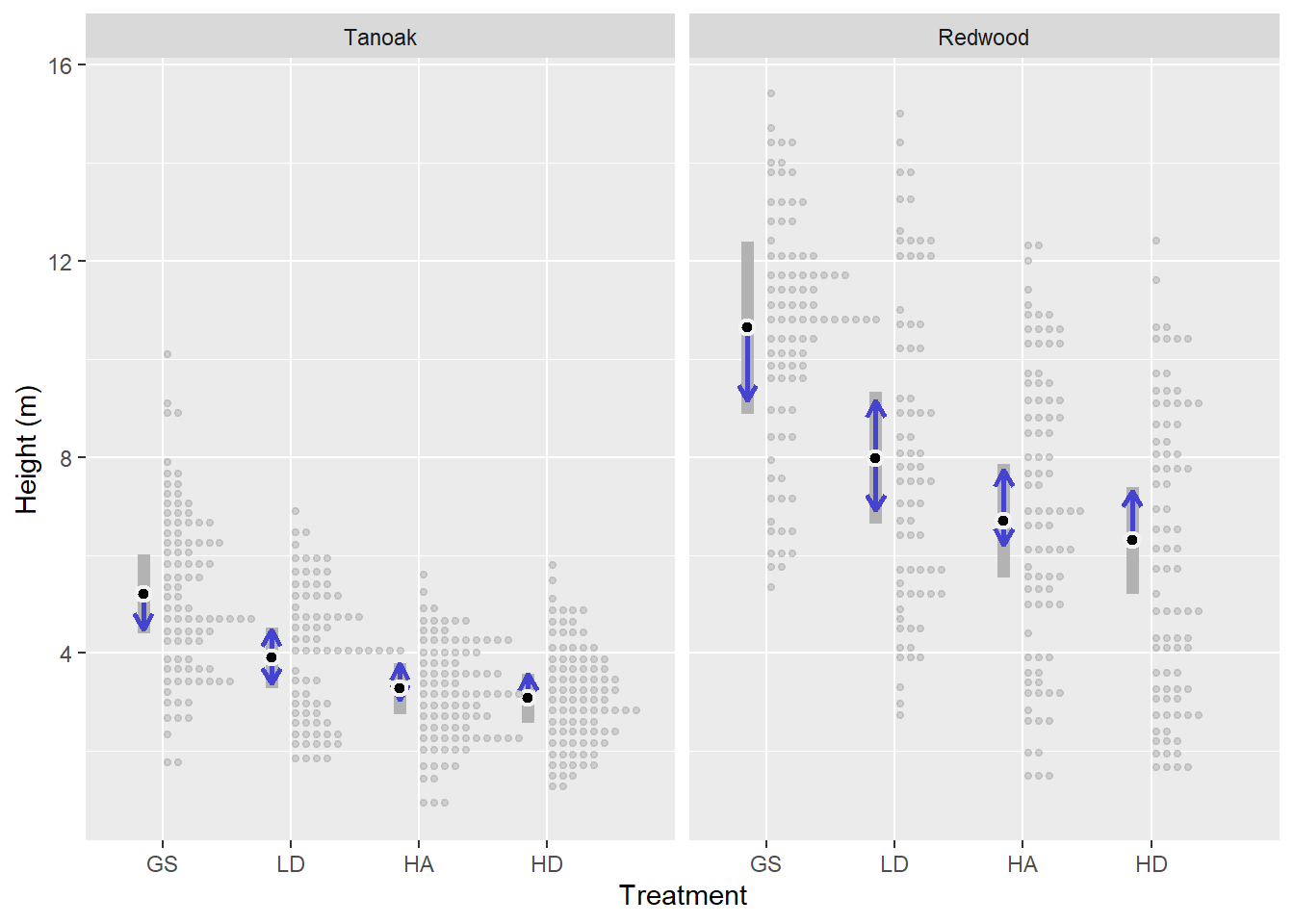
Because the best model did not contain a species x treatment interaction for the mean response, treatment comparisons were parallel between species. The GS treatment resulted in greater heights in year 10 than the other treatments (0.001 < p < 0.05). Predicted mean height for redwood ranged from 10.64 m in the GS treatment to 6.3 m in the HD treatment. For tanoak, predicted mean height ranged from 5.2 m in the GS treatment to 3.08 m in the HD treatment. Predicted mean heights followed the pattern GS > LD > HA ≥ HD (Figure 3.6).
| Spp | Year | Emmean | SE | 95% LCL | 95% UCL |
|---|---|---|---|---|---|
| TO | GS | 5.2 | 0.41 | 4.4 | 6 |
| TO | LD | 3.9 | 0.31 | 3.3 | 4.5 |
| TO | HA | 3.3 | 0.27 | 2.8 | 3.8 |
| TO | HD | 3.1 | 0.25 | 2.6 | 3.6 |
| RW | GS | 10.6 | 0.9 | 8.9 | 12.4 |
| RW | LD | 8 | 0.69 | 6.6 | 9.3 |
| RW | HA | 6.7 | 0.59 | 5.5 | 7.8 |
| RW | HD | 6.3 | 0.55 | 5.2 | 7.4 |
| Spp | Contrast | Emmean | SE | P value |
|---|---|---|---|---|
| TO | GS - LD | 1.3 | 0.5 | 0.05 |
| TO | GS - HA | 1.93 | 0.48 | 0 |
| TO | GS - HD | 2.12 | 0.47 | 0 |
| TO | LD - HA | 0.63 | 0.4 | 0.4 |
| TO | LD - HD | 0.82 | 0.39 | 0.16 |
| TO | HA - HD | 0.19 | 0.36 | 0.95 |
| RW | GS - LD | 2.66 | 1.03 | 0.05 |
| RW | GS - HA | 3.94 | 0.98 | 0 |
| RW | GS - HD | 4.33 | 0.97 | 0 |
| RW | LD - HA | 1.29 | 0.82 | 0.4 |
| RW | LD - HD | 1.68 | 0.81 | 0.16 |
| RW | HA - HD | 0.39 | 0.75 | 0.95 |
3.3 Fuels
Gamma distributed, linear multi-level models, with a log link were used to model fuel load response (Mg ha-1) for all fuel classes. Random intercepts were specified for three levels of nesting, representing sites, macro plots, and transect corners. A hurdle component with logit link was used for predicting zeros in all models except for the duff & litter model. Dispersion components were included where needed, based on AIC model selection. Models were fit separately for pre- and post-PCT fuel measurements. Duff and litter were not measured post-PCT, and vegetation difference was only modeled post-PCT.
family: Gamma(link = "log")
conditional: fuel_load ~ treatment + (1 | site/macro/corner)
\[ Y_i \sim \text{hurdle\_gamma}(\pi_i, \mu_i, \phi_i) \]
\[ \log(\mu_i) = \beta^{\mu}_0 + \beta^{\mu}_{\text{trt}} \cdot \text{Trt}_i + \alpha_{\text{site}[i]} + \alpha_{\text{macro}[i]} + \alpha_{\text{corner}[i]} \]
Any model component not explicitly defined below was modeled with only an intercept:
\[ \text{logit}(\pi_i^\cdot) = \beta^{(\pi,\cdot)}_0 \]
\[ \log(\phi_i^{\cdot}) = \beta^{(\phi,\cdot)}_0 \]
- \(Y_i\): Fuel load (Mg ha-1) for transect \(i\).
- \(\pi_i\): Probability that \(Y_i > 0\), the hurdle component.
- \(\mu_i\): Mean of positive values.
- \(\phi_i\): Dispersion parameter for Gamma distribution.
- \(\alpha_{\cdot}\): Random intercepts for site, macro plot, and corner.
- \(\beta^{\cdot}_{\cdot}\): Fixed effects for intercepts and treatment levels for mean, hurdle, and dispersion components .
3.3.1 Pre-pct
For the Duff & Litter model, there was no hurdle component because there were no zeros in the data, and the dispersion parameter was modeled with only an intercept (see below).
\[ \text{logit}(\pi_i^{\text{dufflitter}}) = \beta^{(\pi,\text{dufflitter})}_0 \]
For the 10-hr fuel model, the hurdle and the dispersion components were modeled as functions of treatment.
\[ \text{logit}(\pi_i^{\text{10hr}}) = \beta^{(\pi,\text{10hr})}_0 + \beta^{(\pi,\text{10hr})}_{\text{trt}} \cdot \text{Trt}_i \]
\[ \log(\phi_i^{\text{10hr}}) = \beta^{(\phi,\text{10hr})}_0 + \beta^{(\phi,\text{10hr})}_{\text{trt}} \cdot \text{Trt}_i \] .
| class | Dispersion (log) | Hurdle (logit) |
|---|---|---|
| Duff & Litter | ~1 | ~0 |
| 1-hr | ~1 | ~1 |
| 10-hr | ~trt | ~trt |
| 100-hr | ~1 | ~1 |
| 1,000-hr | ~1 | ~1 |
| Vegetation | ~1 | ~1 |
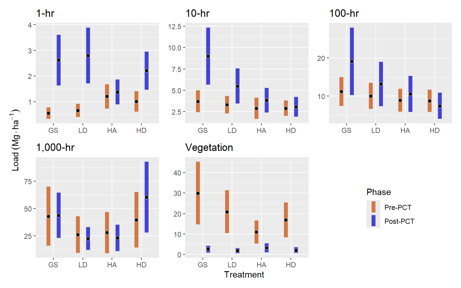
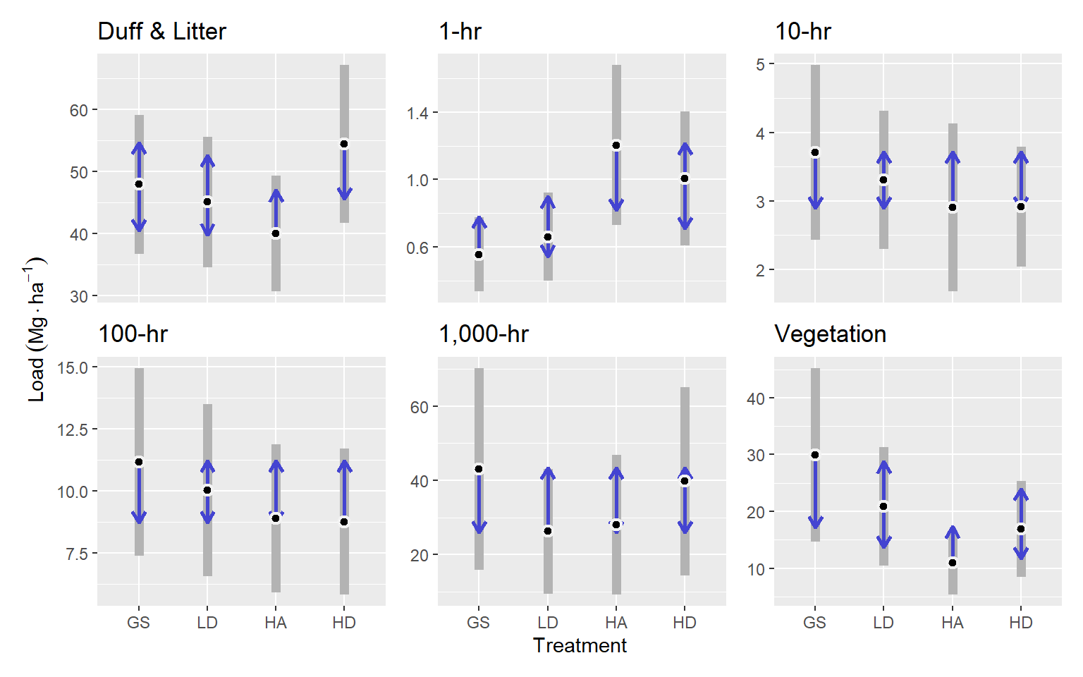
For Duff & Litter, the largest difference was between the HD and HA treatments. The HD treatment had about 54.4 Mg ha-1, and was about 14.39 Mg ha-1 greater than the HA treatment (p = 0.09). Generally, all treatments were similar, with estimated loading of around 47 Mg ha-1.
One-hour fuels were highest in the HA treatment, with an expected value of 1.2 Mg ha-1, which was about Mg ha-1 greater than in the GS treatment (p = 0.03). One-hour fuels in the LD and HD treatments were intermediate but the LD was more similar to the GS and the HD was more similar to the HA treatment.
Ten, hundred and thousand-hour fuels were statistically, very similar across treatments (p ≥ 0.7). Treatment averages had maximum differences of around 1, 3, and 10 Mg ha-1 for ten, hundred, and thousand-hour fuels, respectively.
Vegetative fuel loading was greatest in the GS treatment, with an expected value of 29.94 Mg ha-1, which was about 18.95 Mg ha-1 greater than in the HA treatment (p = 0.05) and LD and HD treatments were intermediate. (Figure 3.7).
| Class | Treat | Emmean | SE | 95% LCL | 95% UCL |
|---|---|---|---|---|---|
| Duff & Litter | gs | 47.93 | 5.69 | 36.76 | 59.09 |
| Duff & Litter | ld | 45.09 | 5.35 | 34.6 | 55.59 |
| Duff & Litter | ha | 40.01 | 4.75 | 30.71 | 49.32 |
| Duff & Litter | hd | 54.4 | 6.46 | 41.74 | 67.06 |
| 1-hr | gs | 0.55 | 0.11 | 0.33 | 0.77 |
| 1-hr | ld | 0.66 | 0.13 | 0.4 | 0.92 |
| 1-hr | ha | 1.2 | 0.24 | 0.73 | 1.68 |
| 1-hr | hd | 1.01 | 0.2 | 0.61 | 1.41 |
| 10-hr | gs | 3.71 | 0.65 | 2.43 | 4.98 |
| 10-hr | ld | 3.31 | 0.52 | 2.3 | 4.32 |
| 10-hr | ha | 2.9 | 0.63 | 1.68 | 4.13 |
| 10-hr | hd | 2.91 | 0.45 | 2.04 | 3.79 |
| 100-hr | gs | 11.17 | 1.92 | 7.41 | 14.93 |
| 100-hr | ld | 10.03 | 1.76 | 6.58 | 13.47 |
| 100-hr | ha | 8.9 | 1.52 | 5.92 | 11.88 |
| 100-hr | hd | 8.76 | 1.49 | 5.84 | 11.69 |
| 1,000-hr | gs | 43.08 | 13.84 | 15.95 | 70.22 |
| 1,000-hr | ld | 26.25 | 8.58 | 9.43 | 43.06 |
| 1,000-hr | ha | 28.06 | 9.58 | 9.29 | 46.83 |
| 1,000-hr | hd | 39.75 | 12.94 | 14.38 | 65.11 |
| Vegetation | gs | 29.94 | 7.78 | 14.69 | 45.19 |
| Vegetation | ld | 20.88 | 5.32 | 10.45 | 31.3 |
| Vegetation | ha | 10.99 | 2.86 | 5.39 | 16.6 |
| Vegetation | hd | 16.86 | 4.32 | 8.4 | 25.32 |
| Class | Contrast | Emmean | SE | P value |
|---|---|---|---|---|
| 1-hr | gs - ha | -0.6491 | 0.24 | 0.033 |
| Vegetation | gs - ha | 18.947 | 7.46 | 0.054 |
| Duff & Litter | ha - hd | -14.3869 | 6.16 | 0.09 |
| 1-hr | ld - ha | -0.5439 | 0.24 | 0.115 |
| 1-hr | gs - hd | -0.4529 | 0.2 | 0.119 |
| Vegetation | ld - ha | 9.8847 | 5.29 | 0.242 |
| Vegetation | gs - hd | 13.0772 | 7.78 | 0.334 |
| 1-hr | ld - hd | -0.3477 | 0.21 | 0.353 |
| Duff & Litter | ld - hd | -9.3078 | 6.38 | 0.463 |
| Duff & Litter | gs - ha | 7.9119 | 5.63 | 0.497 |
| Vegetation | ha - hd | -5.8698 | 4.47 | 0.555 |
| 100-hr | gs - hd | 2.405 | 2.13 | 0.671 |
| Vegetation | gs - ld | 9.0623 | 8.11 | 0.679 |
| 1,000-hr | gs - ld | 16.832 | 15.77 | 0.71 |
| 100-hr | gs - ha | 2.2729 | 2.15 | 0.715 |
| 10-hr | gs - hd | 0.7915 | 0.79 | 0.748 |
| Duff & Litter | gs - hd | -6.475 | 6.53 | 0.755 |
| Duff & Litter | ld - ha | 5.0791 | 5.43 | 0.786 |
| 1,000-hr | gs - ha | 15.0192 | 16.34 | 0.795 |
| 1,000-hr | ld - hd | -13.4991 | 14.91 | 0.802 |
| 10-hr | gs - ha | 0.8008 | 0.9 | 0.809 |
| 1,000-hr | ha - hd | -11.6863 | 15.4 | 0.873 |
| 1-hr | ha - hd | 0.1962 | 0.27 | 0.889 |
| 1-hr | gs - ld | -0.1051 | 0.15 | 0.896 |
| Vegetation | ld - hd | 4.015 | 5.85 | 0.902 |
| 100-hr | ld - hd | 1.2626 | 2.02 | 0.924 |
| 10-hr | ld - hd | 0.3916 | 0.68 | 0.94 |
| 100-hr | ld - ha | 1.1306 | 2.03 | 0.945 |
| 100-hr | gs - ld | 1.1424 | 2.28 | 0.959 |
| 10-hr | ld - ha | 0.401 | 0.81 | 0.96 |
| 10-hr | gs - ld | 0.3998 | 0.83 | 0.963 |
| Duff & Litter | gs - ld | 2.8328 | 5.93 | 0.964 |
| 1,000-hr | gs - hd | 3.3329 | 18.36 | 0.998 |
| 1,000-hr | ld - ha | -1.8127 | 12.21 | 0.999 |
| 100-hr | ha - hd | 0.132 | 1.85 | 1 |
| 10-hr | ha - hd | -0.0094 | 0.77 | 1 |
| Class | Emmean | SE | 95% LCL | 95% UCL |
|---|---|---|---|---|
| Duff & Litter | 46.86 | 4.21 | 38.6 | 55.1 |
| 1-hr | 0.86 | 0.12 | 0.63 | 1.1 |
| 10-hr | 3.21 | 0.28 | 2.65 | 3.8 |
| 100-hr | 9.71 | 1.1 | 7.56 | 11.9 |
| 1,000-hr | 34.29 | 6.31 | 21.93 | 46.6 |
| Vegetation | 19.67 | 3.52 | 12.77 | 26.6 |
3.3.2 Post-pct
After PCT, duff & litter was not modeled, vegetation difference was added. Model selection resulted in somewhat more complex models for dispersion (\(\phi\)) and hurdle (\(\pi\)) components. For 1-hr fuels the dispersion component included treatment and site predictors:
\[ \log(\phi_i^{\text{1hr}}) = \beta^{(\phi,\text{1hr})}_0 + \beta^{(\phi,\text{1hr})}_{\text{trt}} \cdot \text{Trt}_i + \beta^{(\phi,\text{1hr})}_{\text{site}} \cdot \text{Site}_i \] ,
and for 100-hr fuels, the dispersion and hurdle components included treatment and site predictors:
\[ \log(\phi_i^{\text{100hr}}) = \beta^{(\phi,\text{100hr})}_0 + \beta^{(\phi,\text{100hr})}_{\text{trt}} \cdot \text{Trt}_i + \beta^{(\phi,\text{100hr})}_{\text{site}} \cdot \text{Site}_i \]
\[ \text{logit}(\pi_i^{\text{100hr}}) = \beta^{(\pi,\text{100hr})}_0 + \beta^{(\pi,\text{100hr})}_{\text{trt}} \cdot \text{Trt}_i + \beta^{(\pi,\text{100hr})}_{\text{site}} \cdot \text{Site}_i \] .
The dispersion and hurdle components for the rest of the fuel models included only an intercept.
Dispersion models with treatment as the only predictor were included for 1-hr and 100-hr fuel classes. All models included a hurdle portion to model zeros using a logit link. For 100-hr fuels, the hurdle portion included treatment and site as predictors. For the rest, a constant rate of zeros for all observations was used (Table 3.13).
| class | Dispersion (log) | Hurdle (logit) |
|---|---|---|
| 1-hr | ~trt + site | ~1 |
| 10-hr | ~1 | ~1 |
| 100-hr | ~trt + site | ~trt + site |
| 1,000-hr | ~1 | ~1 |
| Vegetation | ~1 | ~1 |
| Vegetation Difference | ~1 | ~1 |
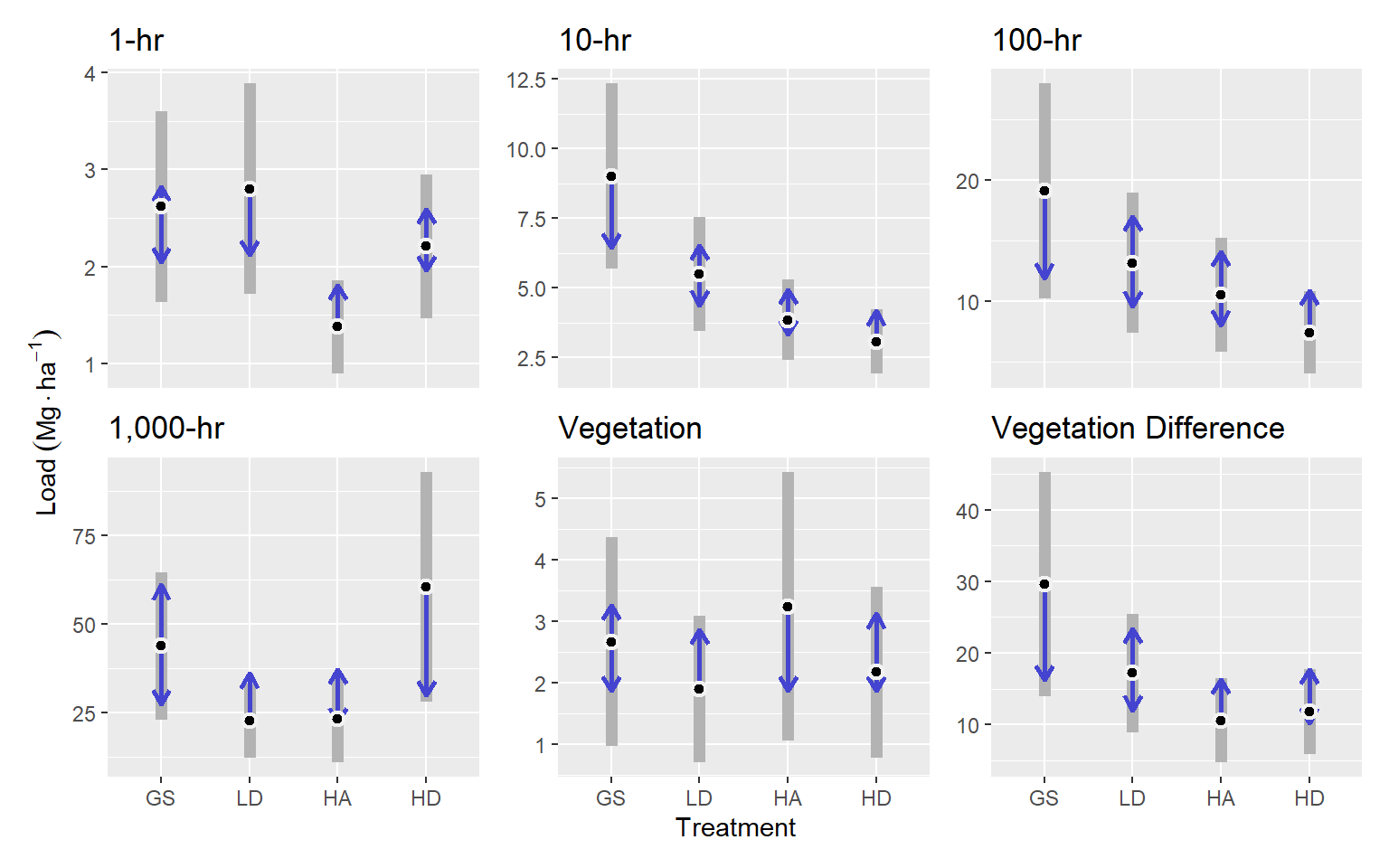
Unlike pre-pct fuel loading which differed little among treatments in terms of fine dead surface fuels, the PCT treatment resulted in additional fine dead surface fuels that differed significantly among treatments. Whereas vegetation fuel loading was reduced and differences between treatments were lessened. Unlike pre-commercial thinning resulted in greater stratification of treatments (Figure 3.8). One-hour fuels for most treatments were around 2.5 Mg ha-1, but the HA treatment was lower than these at about 1.38 Mg ha-1 (p <= ).
The GS treatment had the greatest 10-hr fuel loading with 9 Mg ha-1, which was greater than the LD, HA, and HD treatments by 3.5, 5.15, and 5.94 Mg ha-1, respectively ( p = 0.06, p < 0.001, and p = 0). The LD treatment also had about 2.43 Mg ha-1 more 10-hr fuels that the HD treatment (p = 0.03).
Hundred-hour fuels followed a similar trend as the 10-hr fuels. They were greatest in the GS treatment, with an average of about 19.12 Mg ha-1, which was about 11.69 Mg ha-1 greater than the HD treatment (p = 0.03).
Thousand-hour fuels were greatest in the HD treatment, with an average of about 60.48 Mg ha-1, which was about 37.71 Mg ha-1 greater than the LD and HA treatments (p <= 0.14). The GS treatment was intermediate.
Fuel loading for live vegetation was similar across treatments at around 2.3 Mg ha-1.
The difference in vegetation loading before and after PCT was greatest in the GS treatment at about 29.6 Mg ha-1, which was greater than the HA and HD treatments by about 18 Mg ha-1 (p = 0.09 and p = 0.05, respectively). The LD treatment was intermediate.
| Class | Treat | Emmean | SE | 95% LCL | 95% UCL |
|---|---|---|---|---|---|
| 1-hr | gs | 2.6 | 0.5 | 1.63 | 3.6 |
| 1-hr | ld | 2.8 | 0.55 | 1.71 | 3.9 |
| 1-hr | ha | 1.4 | 0.25 | 0.89 | 1.9 |
| 1-hr | hd | 2.2 | 0.38 | 1.47 | 2.9 |
| 10-hr | gs | 9 | 1.7 | 5.68 | 12.3 |
| 10-hr | ld | 5.5 | 1.05 | 3.44 | 7.6 |
| 10-hr | ha | 3.9 | 0.73 | 2.41 | 5.3 |
| 10-hr | hd | 3.1 | 0.59 | 1.92 | 4.2 |
| 100-hr | gs | 19.1 | 4.52 | 10.26 | 28 |
| 100-hr | ld | 13.2 | 2.97 | 7.36 | 19 |
| 100-hr | ha | 10.5 | 2.41 | 5.81 | 15.3 |
| 100-hr | hd | 7.4 | 1.74 | 4.03 | 10.8 |
| 1,000-hr | gs | 43.9 | 10.61 | 23.08 | 64.7 |
| 1,000-hr | ld | 22.8 | 5.33 | 12.31 | 33.2 |
| 1,000-hr | ha | 23.2 | 6.21 | 11.04 | 35.4 |
| 1,000-hr | hd | 60.5 | 16.55 | 28.05 | 92.9 |
| Vegetation | gs | 2.7 | 0.87 | 0.96 | 4.4 |
| Vegetation | ld | 1.9 | 0.61 | 0.7 | 3.1 |
| Vegetation | ha | 3.2 | 1.12 | 1.06 | 5.4 |
| Vegetation | hd | 2.2 | 0.71 | 0.78 | 3.6 |
| Vegetation Difference | gs | 29.6 | 7.99 | 13.95 | 45.3 |
| Vegetation Difference | ld | 17.2 | 4.22 | 8.89 | 25.4 |
| Vegetation Difference | ha | 10.6 | 2.98 | 4.74 | 16.4 |
| Vegetation Difference | hd | 11.8 | 3.02 | 5.91 | 17.7 |
| Class | Contrast | Emmean | SE | P value |
|---|---|---|---|---|
| 10-hr | gs - hd | 5.94 | 1.46 | 0.00026 |
| 10-hr | gs - ha | 5.15 | 1.43 | 0.00172 |
| 1-hr | ld - ha | 1.42 | 0.43 | 0.00585 |
| 1-hr | gs - ha | 1.24 | 0.39 | 0.00889 |
| 1-hr | ha - hd | -0.83 | 0.26 | 0.00919 |
| 100-hr | gs - hd | 11.69 | 4.16 | 0.02573 |
| 10-hr | ld - hd | 2.43 | 0.87 | 0.02637 |
| Vegetation Difference | gs - ha | 19.03 | 7.48 | 0.05357 |
| 10-hr | gs - ld | 3.5 | 1.41 | 0.06286 |
| Vegetation Difference | gs - hd | 17.78 | 7.55 | 0.08602 |
| 1,000-hr | ld - hd | -37.71 | 17.15 | 0.12359 |
| 1,000-hr | ha - hd | -37.27 | 17.43 | 0.14104 |
| 100-hr | ld - hd | 5.75 | 2.75 | 0.1565 |
| 100-hr | gs - ha | 8.59 | 4.21 | 0.17315 |
| 10-hr | ld - ha | 1.65 | 0.88 | 0.24322 |
| 1,000-hr | gs - ld | 21.12 | 11.6 | 0.26381 |
| 1,000-hr | gs - ha | 20.67 | 12.01 | 0.31242 |
| Vegetation Difference | gs - ld | 12.44 | 7.67 | 0.36644 |
| Vegetation Difference | ld - ha | 6.59 | 4.3 | 0.41898 |
| 1-hr | ld - hd | 0.59 | 0.42 | 0.49237 |
| 100-hr | gs - ld | 5.95 | 4.31 | 0.51297 |
| Vegetation | ld - ha | -1.35 | 0.98 | 0.51617 |
| 100-hr | ha - hd | 3.1 | 2.32 | 0.54089 |
| Vegetation Difference | ld - hd | 5.35 | 4.3 | 0.59869 |
| 10-hr | ha - hd | 0.79 | 0.64 | 0.60281 |
| Vegetation | ha - hd | 1.07 | 0.97 | 0.68792 |
| 1-hr | gs - hd | 0.41 | 0.37 | 0.6903 |
| Vegetation | gs - ld | 0.77 | 0.76 | 0.7434 |
| 100-hr | ld - ha | 2.65 | 2.91 | 0.80002 |
| 1,000-hr | gs - hd | -16.6 | 19.3 | 0.82556 |
| Vegetation | gs - hd | 0.49 | 0.8 | 0.92729 |
| Vegetation | gs - ha | -0.58 | 1.04 | 0.94512 |
| Vegetation | ld - hd | -0.28 | 0.66 | 0.97521 |
| 1-hr | gs - ld | -0.18 | 0.48 | 0.98118 |
| Vegetation Difference | ha - hd | -1.24 | 3.52 | 0.98495 |
| 1,000-hr | ld - ha | -0.45 | 7.78 | 0.99993 |
| Class | Emmean | SE | 95% LCL | 95% UCL |
|---|---|---|---|---|
| 1-hr | 2.3 | 0.36 | 1.5 | 3 |
| 10-hr | 5.4 | 0.84 | 3.7 | 7 |
| 100-hr | 12.6 | 2.2 | 8.3 | 16.9 |
| 1,000-hr | 37.6 | 5.61 | 26.6 | 48.6 |
| Vegetation | 2.5 | 0.65 | 1.2 | 3.8 |
| Vegetation Difference | 17.3 | 3.33 | 10.8 | 23.8 |
3.3.3 Pre-post commercial thinning comparison
The PCT of 10-year-old vegetation dramatically reduced live surface fuels, predictably leading to varying increases in loading across 1- 10- and 100-hr fuels. Specifically PCT led to a small increase in average 100-hr fuel loading, only for the GS treatment, increased 10-hr fuels in the GS and LD treatments, and increased 1-hr fuels for all but the HA treatment (Figure 3.9). However these results were not statistically comparable, due to slightly different model structures.