Code
library(dplyr)
library(tidyr)
library(purrr)
library(ggplot2)
library(forcats)
library(stringr)


library(patchwork)
load("summarize_collected_data.rda")library(dplyr)
library(tidyr)
library(purrr)
library(ggplot2)
library(forcats)
library(stringr)
library(patchwork)
load("summarize_collected_data.rda")We used the line intercept method for tallying fine and coarse woody debris (Brown, 1974; Van Wagner, 1982). In essence, with this technique we are recording the diameters of all dead, downed woody pieces that cross an imaginary sampling plane of a specified length and height. These diameters are convered to crossectional areas which can then be extended to a volume by multiplying by a width. Finally, volume can be converted to mass using specific gravity. This method requires the assumptions that a particle is (1) cylidrical, (2) horizontal, and (3) perpendicular to the sampling plane. While (1) may be a reasonable assumption for many woody particles, 2 and 3 are less likely. For 2, we use a factor which allows us to trade out this assumption, for the assumption that pieces are randomly oriented in the horizontal plane. For 3, we use a correction factor (\(\sec \theta\)) based estimates of average paticle inclination (\(\theta\)).
In practice, the diameter of each piece is not measured, but tallied by size class (up to a certain size, after which it is prudent to measure individual pieces). We used the common time-lag size classes < 0.635 cm; 0.635 - 2.54 cm; and 2.54 - 7.62 cm. All pieces larger than 7.62 cm were measured to the nearest cm. This requires estimating an average diameter (quadratic mean diameter is used) for pieces in each category which can be done using emperical data gathered from specific forest types (Brown, 1974), or estimated from the sampling distribution of the tallies themselves (Van Wagner, 1982). Here we will use the former, with values found in the literature.
The resulting equation for estimating fuel load (Mg/ha) is:
\[Load = \frac{\sum d^2 G k a c}{l} \tag{3.1}\]
where d is diameter (cm), G is specific gravity, k=1.234 is a constant which accounts for random horizontal particle orientation, the density of water and unit conversion factors (Van Wagner, 1982), a is the particle inclination correction factor, c is the transect slope correction factor and l is the transect length. The calculation of a is described above and c is calculated as \(c = \sqrt{1 + (slope ratio)^2}\).
Thus in R, our basic fuel load function will look like this:
simple_load <- function(sum_d2, G, k = 1.234, a, percent_slope, l) {
  c <- sqrt(1 + (percent_slope / 100)^2)
  (sum_d2 * G * k * a * c) / l
}
The “composite” values for G (for both sound and rotten wood), a, and the quadratic mean diameter of a size class (used for d) where provided by Brown (1974) for use when site specific data are unknown. The values given a pertain to “non-slash”. Somewhat larger values are used for slash fuel beds.
lit_particle_params <- dplyr::tribble(
  ~source,
  ~parameter,
  ~onehr,
  ~tenhr,
  ~hundhr,
  ~thoushr_s,
  ~thoushr_r,
  "brown",
  "d2",
  0.10,
  1.86,
  17.81,
  1,
  1,
  "brown",
  "G",
  0.48,
  0.48,
  0.40,
  0.40,
  0.30,
  "brown",
  "a",
  1.13,
  1.13,
  1.13,
  1.00,
  1.00,
  "vanwagtendonk",
  "d2",
  0.12,
  1.28,
  14.52,
  1,
  1,
  "vanwagtendonk",
  "G",
  0.58,
  0.57,
  0.53,
  0.47,
  0.36,
  "vanwagtendonk",
  "a",
  1.03,
  1.02,
  1.02,
  1.02,
  1.02,
)

glebocki_particle_params <- dplyr::tribble(
  ~id,
  ~parameter,
  ~onehr,
  ~tenhr,
  ~hundhr,
  ~thoushr_s,
  ~thoushr_r,
  "85-0405",
  "a",
  1.03,
  1.03,
  1.02,
  1.01,
  1.00,
  "85-0405",
  "d2",
  0.13,
  1.32,
  16.13,
  1,
  1,
  "85-0405",
  "G",
  0.45,
  0.46,
  0.42,
  0.38,
  0.37,
  "85-0607",
  "a",
  1.02,
  1.02,
  1.02,
  1.01,
  1.01,
  "85-0607",
  "d2",
  0.10,
  1.21,
  20.90,
  1,
  1,
  "85-0607",
  "G",
  0.53,
  0.48,
  0.40,
  0.33,
  0.25,
  "85-0809",
  "a",
  1.02,
  1.02,
  1.02,
  1.01,
  1.00,
  "85-0809",
  "d2",
  0.12,
  1.27,
  19.24,
  1,
  1,
  "85-0809",
  "G",
  0.44,
  0.49,
  0.38,
  0.46,
  0.28,
  "85-1011",
  "a",
  1.04,
  1.02,
  1.03,
  1.01,
  1.00,
  "85-1011",
  "d2",
  0.10,
  1.48,
  21.72,
  1,
  1,
  "85-1011",
  "G",
  0.51,
  0.53,
  0.43,
  0.47,
  0.32,
  "85-C",
  "a",
  1.02,
  1.02,
  1.01,
  1.02,
  1.02,
  "85-C",
  "d2",
  0.12,
  1.28,
  17.74,
  1,
  1,
  "85-C",
  "G",
  0.47,
  0.41,
  0.31,
  0.30,
  0.30,
  "9192-0405",
  "a",
  1.02,
  1.02,
  1.01,
  1.01,
  1.00,
  "9192-0405",
  "d2",
  0.12,
  1.45,
  20.68,
  1,
  1,
  "9192-0405",
  "G",
  0.42,
  0.51,
  0.41,
  0.36,
  0.29,
  "9192-0607",
  "a",
  1.03,
  1.05,
  1.02,
  1.01,
  1.01,
  "9192-0607",
  "d2",
  0.12,
  1.52,
  19.42,
  1,
  1,
  "9192-0607",
  "G",
  0.46,
  0.43,
  0.43,
  0.37,
  0.27,
  "9192-0809",
  "a",
  1.03,
  1.04,
  1.01,
  1.01,
  1.00,
  "9192-0809",
  "d2",
  0.11,
  1.44,
  17.69,
  1,
  1,
  "9192-0809",
  "G",
  0.47,
  0.51,
  0.44,
  0.46,
  0.41,
  "9192-1011",
  "a",
  1.02,
  1.03,
  1.01,
  1.00,
  1.00,
  "9192-1011",
  "d2",
  0.13,
  1.64,
  15.32,
  1,
  1,
  "9192-1011",
  "G",
  0.49,
  0.52,
  0.47,
  0.43,
  0.32,
  "9192-C",
  "a",
  1.04,
  1.02,
  1.03,
  1.01,
  1.01,
  "9192-C",
  "d2",
  0.12,
  1.41,
  14.50,
  1,
  1,
  "9192-C",
  "G",
  0.46,
  0.44,
  0.43,
  0.39,
  0.28,
  "97-0809",
  "a",
  1.06,
  1.04,
  1.01,
  1.01,
  1.00,
  "97-0809",
  "d2",
  0.12,
  1.81,
  20.35,
  1,
  1,
  "97-0809",
  "G",
  0.46,
  0.52,
  0.46,
  0.47,
  0.45,
  "97-1011",
  "a",
  1.11,
  1.29,
  1.01,
  1.01,
  1.04,
  "97-1011",
  "d2",
  0.11,
  1.46,
  18.49,
  1,
  1,
  "97-1011",
  "G",
  0.48,
  0.56,
  0.46,
  0.42,
  0.41,
  "97-C",
  "a",
  1.02,
  1.01,
  1.03,
  1.08,
  1.00,
  "97-C",
  "d2",
  0.12,
  1.40,
  18.63,
  1,
  1,
  "97-C",
  "G",
  0.39,
  0.36,
  0.44,
  0.37,
  0.37,
)

# Currently this function summarizes data across all Glebocki plots, I could #
# adapt this later if I only want to include some plots.
summarize_glebocki <- function(data) {
  data |>
    dplyr::group_by(parameter) |>
    dplyr::summarize(across(where(is.numeric), ~ round(mean(.x), 2))) |>
    dplyr::mutate(source = "glebocki", .before = 1)
}

lit_particle_params <- dplyr::bind_rows(
  lit_particle_params,
  summarize_glebocki(glebocki_particle_params)
) |>
  dplyr::arrange(parameter)

get_particle_params <- function(params = lit_particle_params, source) {
  params[params$source == source, !names(params) %in% "source"] |>
    pivot_longer(-c(parameter), names_to = "class") |>
    pivot_wider(names_from = parameter, values_from = value)
}
A study of Sierra Nevada conifers found these values to vary by species, and estimates of fuel loading ranged from 40% less to 8% more than when using those suggested by Brown (1974). A study of young, treated redwood and Douglas-fir stands (Glebocki, 2015) found similar values for G to those of Brown (1974), and values for a much closer to those of Van Wagtendonk et al. (1996) (Table 3.1). Note that the 1’s for thousand hr fuel diameters reflect that the diameters, not counts were measured in the field.
| source | parameter | onehr | tenhr | hundhr | thoushr_s | thoushr_r |
|---|---|---|---|---|---|---|
| brown | G | 0.48 | 0.48 | 0.40 | 0.40 | 0.30 |
| vanwagtendonk | G | 0.58 | 0.57 | 0.53 | 0.47 | 0.36 |
| glebocki | G | 0.46 | 0.48 | 0.42 | 0.40 | 0.33 |
| brown | a | 1.13 | 1.13 | 1.13 | 1.00 | 1.00 |
| vanwagtendonk | a | 1.03 | 1.02 | 1.02 | 1.02 | 1.02 |
| glebocki | a | 1.04 | 1.05 | 1.02 | 1.02 | 1.01 |
| brown | d2 | 0.10 | 1.86 | 17.81 | 1.00 | 1.00 |
| vanwagtendonk | d2 | 0.12 | 1.28 | 14.52 | 1.00 | 1.00 |
| glebocki | d2 | 0.12 | 1.44 | 18.52 | 1.00 | 1.00 |
The above information will allow us to calculate fuel loading for fine and coarse woody debris. First we’ll load our data and get the FWD (and the fuel particle parameters) in a long format for easier calculations.
Two transects are missing slope. I’m giving them a slope of 0 for now.
# use this to reduce the amount of typing when referring to transects
transectid <- c("phase", "site", "treatment", "corner", "azi")

fwd <- d$transects |>
  select(all_of(transectid), slope, matches("one|ten|hun")) |>
  mutate(slope = if_else(is.na(slope), 0, slope)) |>
  # join transect lengths for one ten and hundred hour counts
  left_join(select(d$plots, phase, site, treatment, matches("one|ten|hun"))) |>
  # move onehr, tenhr, etc to new column and create new columns for transect
  # length and particle counts
  pivot_longer(
    matches("count|len"),
    names_to = c("class", ".value"),
    names_sep = "_"
  ) |>
  left_join(get_particle_params(source = "glebocki")) |>
  mutate(
    load = simple_load(
      sum_d2 = count * d2,
      l = length,
      percent_slope = slope,
      G = G,
      a = a
    )
  ) |>
select(-c(G, a))Coarse woody debris is already in a long format so we don’t need to pivot longer, but we will summarize the data for each transect by getting the sum of squared diameters. This differs from the fine woody data because we have actual diameters instead of counts, each diameter corresponds to a single observation.
We only have parameters for “sound” and “rotten” particles, so anything over decay class 3 will be considered “rotten”. Finally, we need to join in transect slopes, and transect lengths.
I’m setting a couple of missing slope to zero.
TODO: Make missing transects be explicit zeros
cwd <- d$coarse_woody |>
  mutate(class = if_else(decay > 3, "thoushr_r", "thoushr_s")) |>
  group_by(phase, site, treatment, corner, azi, class) |>
  # named count to match fwd table, but these are actually summed d^2
  summarize(
    sum_d2 = sum(dia^2),
    count = n(),
    med_d = median(dia),
    .groups = "drop"
  ) |>
  # make missing cwd explicit
  right_join(d$transects[c(transectid, "slope")]) |>
  replace_na(
    list(med_d = 0, sum_d2 = 0, count = 0, slope = 0, class = "thoushr_s")
  ) |>
  left_join(d$plots[c("phase", "site", "treatment", "thoushr_length")]) |>
  left_join(get_particle_params(source = "glebocki")) |>
  mutate(
    load = simple_load(
      sum_d2 = sum_d2,
      l = thoushr_length,
      percent_slope = slope,
      G = G,
      a = a
    )
  ) |>
select(-c(G, a, d2), length = thoushr_length)We measured total duff/litter depth, and then estimated a percent of this depth that would be classified as litter. Litter is any leaf material not classified as a 1-hr fuel, that has not yet begun to break down. Particles that were very dark in color and that were broken into smaller pieces than when they had originally fallen were classified as duff.
Duff and litter were measured at two locations along each transect, for a total of 16 measurements per plot.
To convert these depths to load values we use a depth to load equation. Finney & Martin (1993) found a wide variability in the bulk densities of samples, suggesting that simply using the average bulk density should be sufficient, as opposed to calculating bulk densities based on strata depth or differentiating between duff and litter.
| Source | Description | Load Mg ha-1 cm-1 |
|---|---|---|
| Finney & Martin (1993) | Annadel SP & Humboldt Redwoods SP (rw dbh <= 60 in) | 7.15 |
| Kittredge (1940) | plantation redwoods | 6.80 |
| Stuart, J.D. 1985, Unpubl. in Finney & Martin (1993) | Redwoods SP, (mean of duff & litter) | 9.25 |
| Van Wagtendonk et al. (1998) | Avg. for Sierra Nevada conifers | 16.24 |
| Nives (1989) | Redwood NP, Lost Man Cr., Redwood Cr. | 2.42 |
| Krieger et al. (2020) | No ref. cited, 2.75 and 5.5 lbs/ft3 litter and duff resp. | 6.60 |
| Valachovic et al. (2011) | Tanoak-Douglas-fir, litter only, Humboldt County | 0.93 |
On average, we have about 50% litter and a depth of about 6.2 cm. If we use the mean of the first 3 rows in Table 3.2, an average depth to load multiplier for redwood forests (with 50% litter) is 7.73 Mg ha-1 cm-1.
dufflitter |>
  group_by(treatment) |>
  summarize(
    avg_pct_litter = mean(
      litter_depth / (duff_depth + litter_depth),
      na.rm = TRUE
    ),
    avg_total_depth = mean(duff_depth + litter_depth)
  )
# A tibble: 4 × 3
treatment avg_pct_litter avg_total_depth
<chr> <dbl> <dbl>
1 gs 0.689 14.2
2 ha 0.695 7.94
3 hd 0.610 10.4
4 ld 0.613 12.4 dufflitter <- dufflitter |>
mutate(
load = (duff_depth + litter_depth) * 7.73
)We based our data collection on the Firemon protocol, which determines vegetative fuel loading by multiplying estimated percent cover by height by a constant bulk densities of 8 and 18 t/ha/m for herbaceous and shrub components, respectively.
Here I want to standardize the data so that heights are all zero (instead of NA), if percent cover for live and dead were both zero. Also, I want total percent cover, with total proportion dead.
Theoretically, with the Firemon protocol, total percent cover could be greater than 100, because live and dead percent covers are assessed separately. In practice, sum of live and dead cover was over 100 percent.
veg_match <- "woody|herb|avg_w_ht|avg_h_ht|species"

veg <- d$transects |>
  select(all_of(transectid), slope, matches(veg_match)) |>
  pivot_longer(
    !c(any_of(transectid), slope),
    names_to = c(".value", "station"),
    names_pattern = "(\\w+)([12])"
  ) |>
  # there was some inconsistency in whether heights were zero or blank if no veg
  # was present, here I sort that out.
  # We are interested in total load, but the dead component has implications for
  # fuel moisture. We recorded percent cover of live and dead separately, so
  # here i calculate a total and proportion dead.
  mutate(
    woody_ht = if_else(live_woody == 0 & dead_woody == 0, 0, avg_w_ht),
    herb_ht = if_else(live_herb == 0 & dead_herb == 0, 0, avg_h_ht),
    woody_load = ((live_woody + dead_woody) / 100) * woody_ht * 18,
    woody_p_dead = if_else(
      woody_load == 0,
      0,
      dead_woody / (live_woody + dead_woody)
    ),
    herb_load = ((live_herb + dead_herb) / 100) * herb_ht * 8,
    herb_p_dead = if_else(
      herb_load == 0,
      0,
      dead_herb / (live_herb + dead_herb)
    )
  ) |>
  select(!matches("live_|dead_|avg_"), woody_ht, herb_ht) |>
  pivot_longer(
    matches("woody|herb"),
    names_to = c("class", ".value"),
    names_pattern = "(woody|herb)_(.*)"
)Now we can join results for fine woody debris, coarse woody debris, litter, and duff into a single dataframe.
Vegetation and duff/litter first need to be summarized to the transect level.
dufflitter_load <- dufflitter |>
  group_by(pick(all_of(transectid))) |>
  summarize(class = "dufflitter", load = mean(load))

veg_load <- veg |>
  group_by(pick(all_of(transectid)), class) |>
  summarize(load = mean(load))

fwd_load <- fwd |> select(all_of(transectid), class, load)
cwd_load <- cwd |> select(all_of(transectid), class, load)

total_load <- bind_rows(dufflitter_load, veg_load, fwd_load, cwd_load) |>
  ungroup()
John Stuart measured old-growth forest fuels in in Bull Creek Drainage of Humboldt Redwood State Park, approximately 30 km inland from the coast. Overstory BA was about 66 m2ha-1. Plots were classifed based on their overstory/understory species as one of:
Finney & Martin (1993) measured fuels at two loacations. In Annadel SP with 30-40% slopes and 45 - 60 m2ha-1 of trees approximate 120 years old. At RW SP, BA was between 20 and 60 m2ha-1 that sprouted after harvest and were around 90 years old.
Kittredge (1940) studied duff and litter in redwood plantations with an average total depth of 4 cm.
Valachovic et al. (2011) measured surface fuels in Douglas-fir-tanoak forests from Sonoma to northern Humboldt counteis. The values shown are from across this range.
| source | low | high | |
|---|---|---|---|
| litter | valachovic | 2.9 | 4.7 |
| dufflitter | thisstudy | 40.2 | 55.0 |
| finney | 29.0 | 55.0 | |
| kittredge | 24.0 | 24.0 | |
| stuart | 30.9 | 73.6 | |
| onehr | thisstudy | 0.6 | 1.2 |
| valachovic | 2.0 | 3.4 | |
| stuart | 0.9 | 2.1 | |
| tenhr | thisstudy | 2.9 | 3.7 |
| valachovic | 2.5 | 6.1 | |
| stuart | 3.5 | 6.4 | |
| hundhr | thisstudy | 9.5 | 11.8 |
| valachovic | 3.1 | 7.6 | |
| stuart | 2.8 | 7.5 | |
| onetenhundhr | thisstudy | 13.4 | 16.1 |
| finney | 9.0 | 20.0 | |
| valachovic | 9.0 | 15.5 | |
| stuart | 8.0 | 13.4 |
| source | low | high | |
|---|---|---|---|
| thoushr_s | thisstudy | 19.4 | 40.9 |
| valachovic | 4.9 | 76.7 | |
| stuart | 5.0 | 117.4 | |
| thoushr_r | thisstudy | 23.0 | 59.0 |
| valachovic | 3.1 | 35.2 | |
| stuart | 0.5 | 46.7 | |
| thoushr | thisstudy | 35.3 | 44.9 |
| finney | 0.0 | 264.0 | |
| valachovic | 18.3 | 85.9 | |
| stuart | 5.6 | 126.3 | |
| veg_woody | thisstudy | 12.4 | 37.8 |
| stuart | 0.1 | 5.6 | |
| veg_herb | thisstudy | 0.2 | 0.5 |
fig_labels <- labeller(
  class = c(
    dufflitter = "Duff & Litter",
    herb = "Herbaceous Veg.",
    hundhr = "100-hr",
    onehr = "1-hr",
    tenhr = "10-hr",
    thoushr_r = "1000-hr Rotten",
    thoushr_s = "1000-hr Sound",
    woody = "Woody Veg."
  ),
  phase = c(
    prepct = "Pre-pct",
    postpct = "Post-pct"
  )
)

p1 <- total_load |>
  summarize(
    .by = c(phase, treatment, class),
    mean = mean(load, na.rm = TRUE),
    se = mean / sqrt(sum(!is.na(load)))
  ) |>
  filter(str_detect(class, "one|ten|hund|duff")) |>
  mutate(
    phase = factor(phase, levels = c("prepct", "postpct")),
    treatment = factor(treatment, levels = c("gs", "ld", "ha", "hd")),
    class = factor(
      class,
      levels = c(
        "onehr",
        "tenhr",
        "hundhr",
        "dufflitter",
        "thoushr_r",
        "thoushr_s",
        "woody",
        "herb"
      )
    )
  ) |>
  filter(!phase == "postpct" | !class == "dufflitter") |>
  ggplot(aes(treatment, mean)) +
  geom_pointrange(aes(ymin = mean - se, ymax = mean + se)) +
  facet_grid(class ~ phase, scales = "free_y", labeller = fig_labels)

p2 <- total_load |>
  summarize(
    .by = c(phase, treatment, class),
    mean = mean(load, na.rm = TRUE),
    se = mean / sqrt(sum(!is.na(load)))
  ) |>
  filter(str_detect(class, "thous|wood|herb")) |>
  mutate(
    phase = factor(phase, levels = c("prepct", "postpct")),
    treatment = factor(treatment, levels = c("gs", "ld", "ha", "hd")),
    class = factor(
      class,
      levels = c(
        "onehr",
        "tenhr",
        "hundhr",
        "dufflitter",
        "thoushr_r",
        "thoushr_s",
        "woody",
        "herb"
      )
    )
  ) |>
  filter(!phase == "postpct" | !class == "dufflitter") |>
  ggplot(aes(treatment, mean)) +
  geom_pointrange(aes(ymin = mean - se, ymax = mean + se)) +
  facet_grid(class ~ phase, scales = "free_y", labeller = fig_labels)

p1 + p2 + plot_layout(guides = "collect")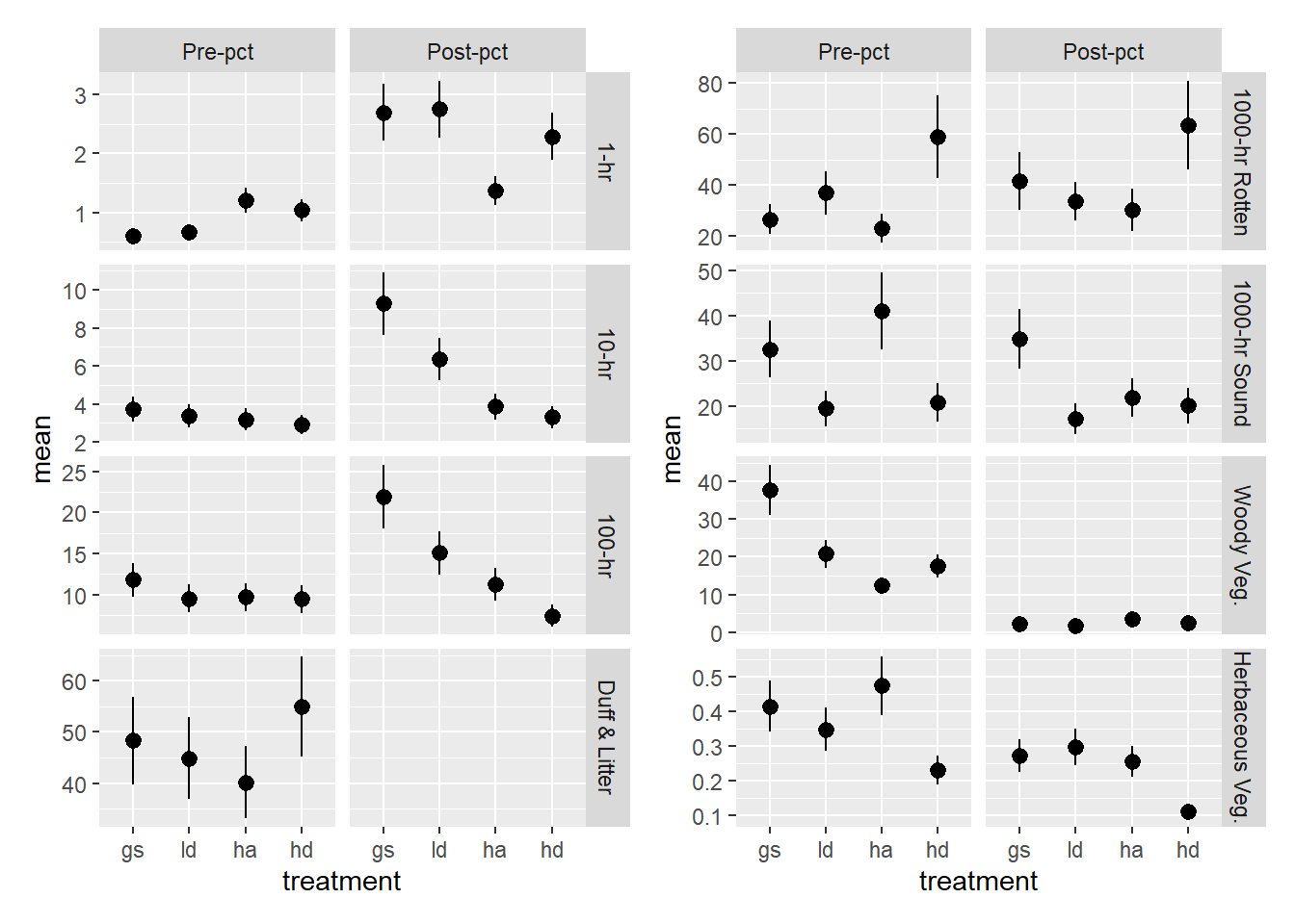
I want to reduce the number of variables that I have to deal with. I will combine the woody and herbaceous veg and also the sound and rotten 1,000-hr fuels.
# To reduce the number of variables, combine sound and rotten coarse wood and
# combine woody and herbaceous veg
tl <- total_load |>
  pivot_wider(names_from = class, values_from = load) |>
  mutate(
    thoushr = rowSums(pick(c(thoushr_s, thoushr_r)), na.rm = TRUE),
    veg = rowSums(pick(c(woody, herb)), na.rm = TRUE),
    .keep = "unused"
  ) |>
  mutate(
    treatment = forcats::fct_relevel(treatment, c("gs", "ld", "ha", "hd"))
)in order to make comparisons, I want to know if any transects had different azimuths in the pre and post pct measure. It looks like there are 11 transects that were measured on a different azimuth. This is about 9% of the data.
tl |>
  select(phase, site, treatment, corner, azi) |>
  group_by(site, treatment, corner, azi) |>
  mutate(n = n()) |>
  filter(n == 1) |>
  arrange(site, treatment, corner, phase) |>
  print(n = Inf)
# A tibble: 22 × 6
# Groups: site, treatment, corner, azi [22]
phase site treatment corner azi n
<chr> <chr> <fct> <chr> <dbl> <int>
1 postpct camp6 gs e 0 1
2 prepct camp6 gs e 225 1
3 postpct camp6 gs w 39 1
4 prepct camp6 gs w 45 1
5 postpct camp6 hd w 42 1
6 prepct camp6 hd w 48 1
7 postpct waldon gs n 262 1
8 prepct waldon gs n 248 1
9 postpct waldon ha ne 290 1
10 prepct waldon ha ne 274 1
11 postpct waldon ha sw 35 1
12 prepct waldon ha sw 6 1
13 postpct waldos gs ne 168 1
14 prepct waldos gs ne 180 1
15 postpct waldos ha ne 178 1
16 prepct waldos ha ne 180 1
17 postpct waldos hd se 287 1
18 prepct waldos hd se 270 1
19 postpct waldos hd sw 356 1
20 prepct waldos hd sw 0 1
21 postpct whiskey hd s 36 1
22 prepct whiskey hd s 42 1For the post pct data, one variable that I would like to analyze is the difference between pre and post vegetation. The difference represents the resulting slash. This should only be calculated for transects that were measured on the same azimuth before and after pct
tl2 <- tl |>
  group_by(site, treatment, corner, azi) |>
  arrange(site, treatment, corner, azi, phase) |>
  mutate(veg_diff = lead(veg) - veg) |>
ungroup()Our combined duff-litter depths were comparable to other studies, resulting in comparable loading for litter and duff.
Onehr fuels were lower than then other redwood study and that found in Douglas-fir/tanoak forests, which is somewhat supprising.
Hundhr fuels were higher in our stands. This makes sense given the logging.
Total fine fuel loading (onetenhundhr) was similar to other studies, but apprently with more hundhr particles.
Thoushr fuels are notoriously variable. Those on our sites were more consistent and within the middle of the range of other reported values.
Woody vegetation was much higher than in the one other reported study. That study was in old-growth redwoods. Our values include tree sprout vegetation, which can be several times taller than evergreen huckleberry and much bushier than understory tanoak saplings. Stuart did mention the presence of “nearly inpenetrable [evergreen huckleberry] thickets.” Stuart (1985) found good correlation of live fuels (which included leaves and “twigs”) with basal diamter for both huckleberry and tanoak saplings. The simple scaling factor and/or the occular estimates we used may be biased.
I’ll Save this data so it can be used in subsequent analysis.
write.csv(total_load, file = "transect_fuel_load.csv")
write.csv(dufflitter, file = "sampling_cylinder_dufflitter.csv")
If you are JD Wilder, you should download this csv file that has all of the fuel loads summarized by transect for pre- and post-pct.
Duff and litter depths were sampled at two places along each transect, here is a csv that has per-cylinder depths and the (crudely calculated) load.
total_load <- tl2

save(dufflitter, fwd, cwd, veg, total_load, file = "calculate_fuel_load.rda")