8  Sprout data exploration

First, we’ll load some libraries and our data.

library(ggdist)
library(ggridges)
library(patchwork)
library(ggplot2)
library(dplyr)
library(tidyr)
library(forcats)

load("wrangled_sprouts.rda")
source("./scripts/rnd_color_brewer.r")

8.1 Objectives

1. For each species/treatment combination, is there a difference in height increment between the first and second periods?
2. Is there a treatment difference in redwood or tanoak sprout heights at year 10, if so, what is the magnitude of the difference?

8.2 Visualize data

8.2.1 Tree heights

The following figures reveal possible trends in the raw data.

8.2.1.1 Species/treatment/year

Redwood is consistently taller than tanoak, and the GS treatment confers the greatest advantage to redwood.

Across all treatments, it is also interesting to note that over times, the height distributions, especially for redwood, seem to becoming more multi-modal and more widely distributed. This could be due to site or plot effects, or to microsite (within plot) effects, but it is not immediately clear why this diverging performance should be so apparent with redwood and not tanoak.

#|
#| message: false

species_labels <- c(LIDE = "Tanoak", SESE = "Redwood")
year_labels <- c(`1` = "Year 1", `5` = "Year 5", `10` = "Year 10")
plot_labels <- labeller(
  spp = species_labels,
  year = year_labels
)


sprouts |>
  lengthen_data("ht") |>
  ggplot(aes(ht, treat, color = treat, fill = treat)) +
  scale_y_discrete(expand = c(0, 0)) +
  scale_x_continuous(expand = c(0, 0)) +
  coord_cartesian(clip = "off") +
  geom_dots(binwidth = unit(0.019, "npc")) +
  facet_grid(vars(spp), vars(year), scales = "free_x", labeller = plot_labels) +
  labs(x = "Height (m)", y = "Treatment") +
  scale_color_brewer(palette = "Set2", aesthetics = c("color", "fill")) +
  theme(legend.position = "bottom")

Warning: The provided binwidth will cause dots to overflow the boundaries of the
geometry.
→ Set `binwidth = NA` to automatically determine a binwidth that ensures dots
  fit within the bounds,
→ OR set `overflow = "compress"` to automatically reduce the spacing between
  dots to ensure the dots fit within the bounds,
→ OR set `overflow = "keep"` to allow dots to overflow the bounds of the
  geometry without producing a warning.
ℹ For more information, see the documentation of the `binwidth` and `overflow`
  arguments of `?ggdist::geom_dots()` or the section on constraining dot sizes
  in vignette("dotsinterval") (`vignette(ggdist::dotsinterval)`).
The provided binwidth will cause dots to overflow the boundaries of the
geometry.
→ Set `binwidth = NA` to automatically determine a binwidth that ensures dots
  fit within the bounds,
→ OR set `overflow = "compress"` to automatically reduce the spacing between
  dots to ensure the dots fit within the bounds,
→ OR set `overflow = "keep"` to allow dots to overflow the bounds of the
  geometry without producing a warning.
ℹ For more information, see the documentation of the `binwidth` and `overflow`
  arguments of `?ggdist::geom_dots()` or the section on constraining dot sizes
  in vignette("dotsinterval") (`vignette(ggdist::dotsinterval)`).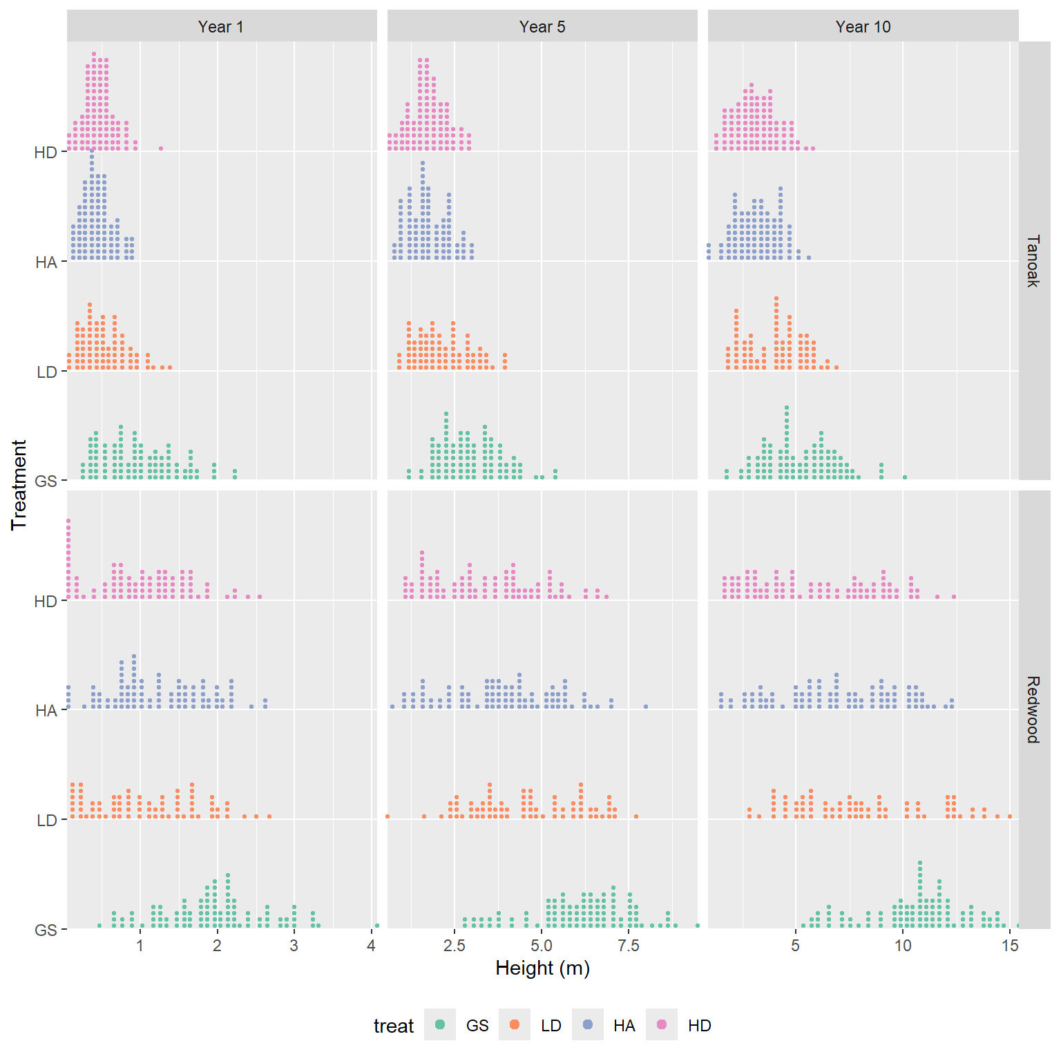

Figure 8.1: Raw sprout heights for redwood and tanoak in four different harvest treatments, at three measurement periods over 10 years. Note the difference in x-axis scales.

This plot shows the raw data collected for ~100 redwood and tanoak sprout clumps in each of four harvest treatments. There is a clear increasing trend with year. The height distribution of redwood is much more dispersed than tanoak. The dispersion of both species increases with year. Redwood are consistently taller. There appears to be an increasing trend in height in treatments where GS > LD > HA > HD.

sprouts |>
  lengthen_data("ht") |>
  ggplot(aes(
    x = ht,
    y = fct_relevel(treat, treat_order),
    color = factor(spp, levels = c("SESE", "LIDE"))
  )) +
  scale_y_discrete(expand = c(0, 0)) +
  scale_x_continuous(expand = c(0, 0)) +
  coord_cartesian(clip = "off") +
  geom_density_ridges(alpha = .3, size = 1) +
  facet_grid(year ~ ., labeller = plot_labels) +
  labs(x = "Height (m)", y = "Treatment") +
  scale_color_brewer(
    palette = "Set2",
    name = "Species",
    labels = species_labels
  )

Warning in geom_density_ridges(alpha = 0.3, size = 1): Ignoring unknown
parameters: `size`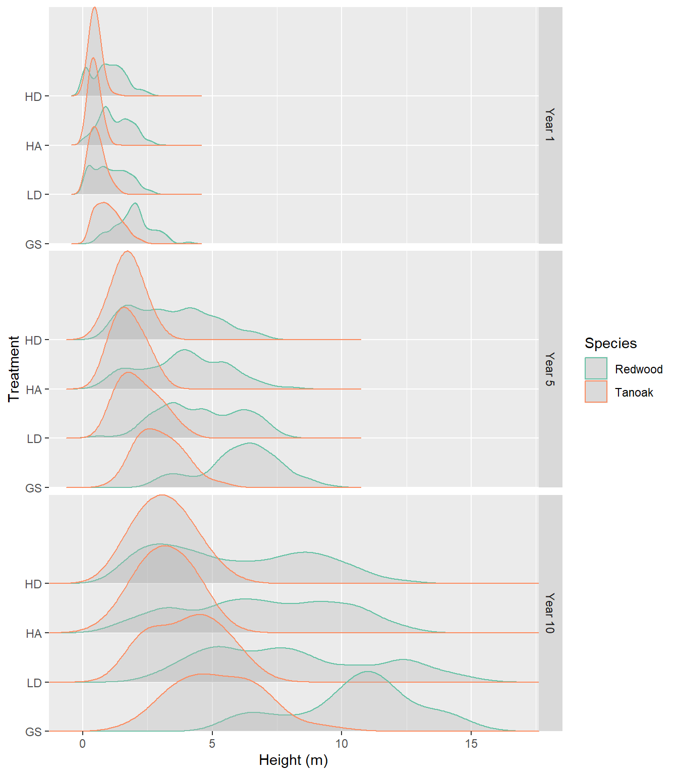

Figure 8.2: Density plots of raw sprout heights for redwood and tanoak in four different harvest treatments, at three measurement periods over 10 years.

8.2.1.2 Species/year/SDI

Figure 8.3 shows that above around 400 SDI, tree heights level off. It also implies a steady decrease in height from 0 to around 400 SDI. The strength of the relationship appears to be increasing over time, particularly for redwood.

sprouts |>
  lengthen_data("ht") |>
  ggplot(aes(sdi_init, ht, color = factor(year))) +
  geom_point(alpha = 0.5) +
  geom_smooth(span = 1.2) +
  facet_wrap(~spp) +
  scale_color_brewer(palette = "Set2")

`geom_smooth()` using method = 'loess' and formula = 'y ~ x'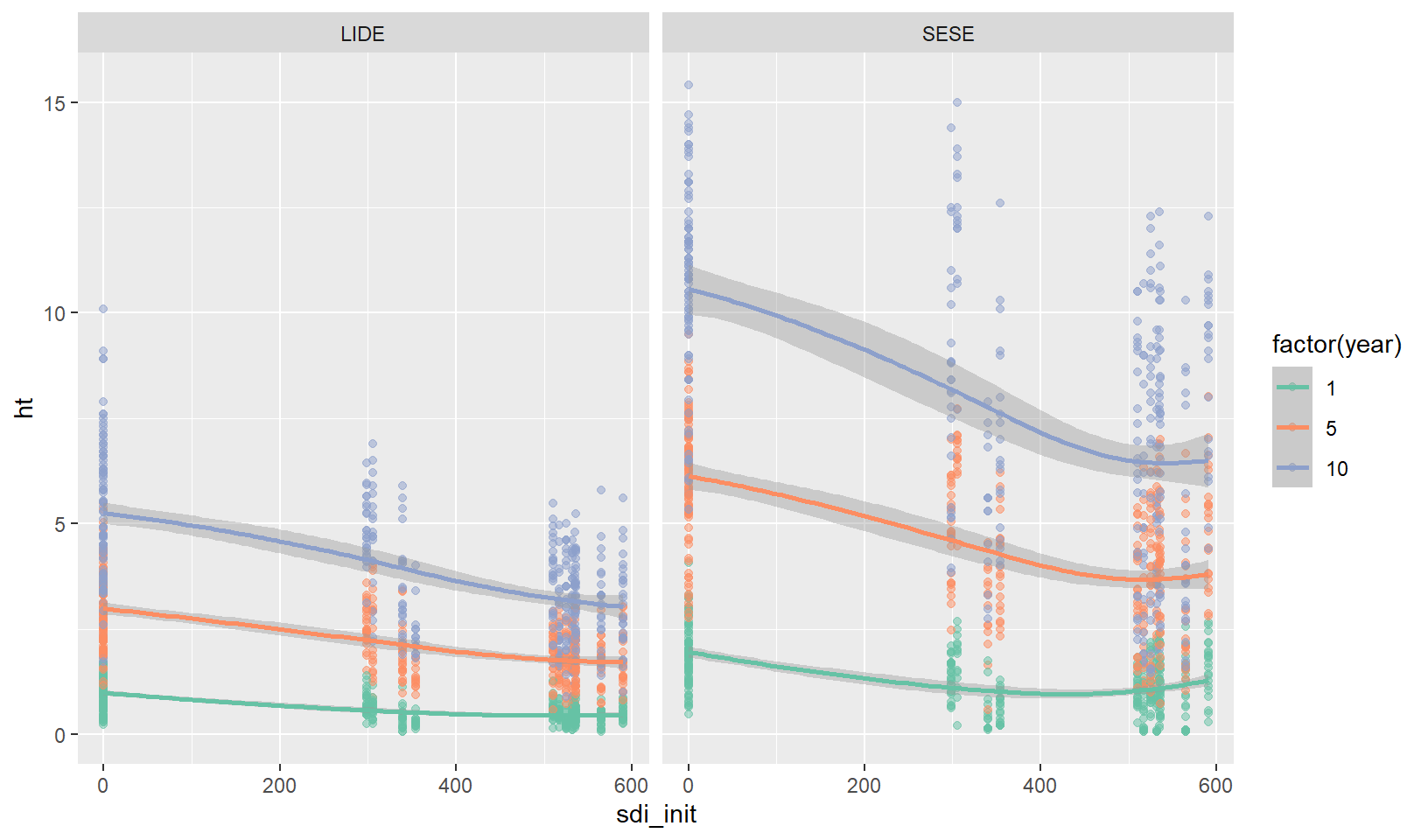

Figure 8.3: SDI vs HT for both species, across measurement years.

8.2.1.3 Species/site/plots

Lets see what the variability among sites and plots looks like, I’ll focus on year 10 only.

Figure 8.4 reveals some differences between sites, particularly for redwoods. Waldo North tends to have larger redwoods and Camp 6 has a large proportion of smaller redwoods.

Figure 8.5 shows that much of the difference in sites has to do with one outlier plot within a site, and less about general site trends. We should expect plots to capture a portion of the variance. Most notable is the plot level difference between redwood and tanoak. For redwood, the large ammount of within plot variability combined with the between plot variability obscures the treatment (and site) effect. If you squint, there appears to be a similar overall pattern between redwood and tanoak repsonse to treatment, but it appears they respond differentially to certain plots.

sprouts |>
  ggplot(aes(ht10, site, fill = spp)) +
  stat_slab(aes(thickness = after_stat(pdf * n)), alpha = 0.6, scale = 0.7) +
  stat_dotsinterval(side = "bottom", scale = 0.7, slab_color = NA) +
  scale_fill_brewer(palette = "Set2") +
  labs(x = "year 10 height (m)", y = NULL, fill = "species")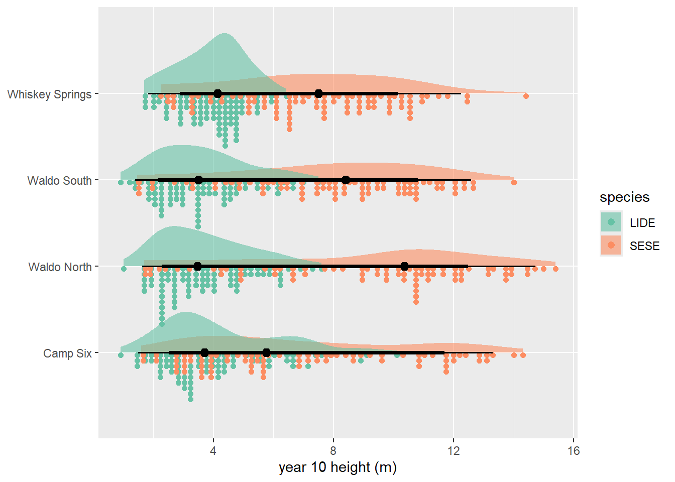

Figure 8.4: Distribution of heights at year 10 at each site for two species. Slabs are normalized by sample size to reflect the raw data, plotted as dots below.

sprouts |>
  mutate(treat = fct_relevel(treat, treat_order)) |>
  ggplot(aes(
    ht10,
    site,
    fill = treat,
  )) +
  stat_slab(aes(thickness = after_stat(pdf * n)), alpha = 0.5, scale = 0.7) +
  stat_pointinterval(
    position = position_dodge(width = 0.5, preserve = "single")
  ) +
  scale_color_brewer(palette = "Set2") +
  facet_wrap(~spp) +
  theme(legend.position = "bottom") +
  labs(y = NULL, x = "year 10 height (m)", fill = "treatment")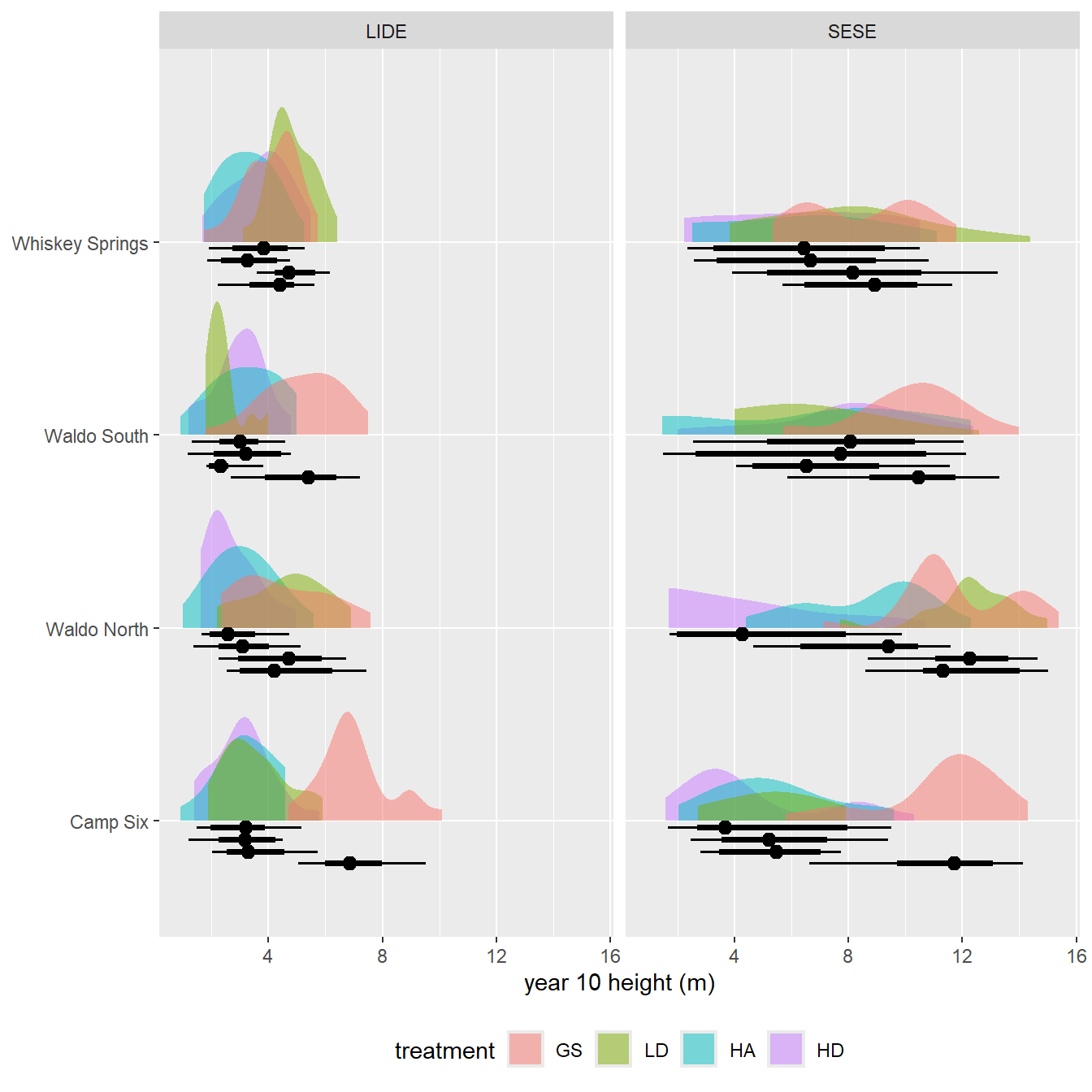

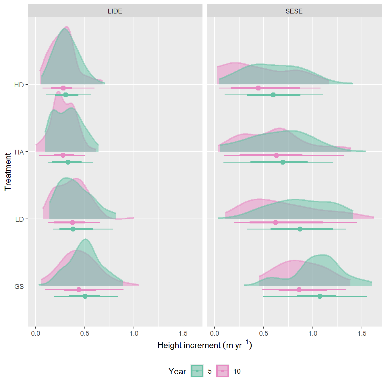
Figure 8.5: Same as for Figure 8.4, but for each plot (Site/treatment interaction). Grouped by treatment.

8.2.2 Height increments

Height increments contain similar information as heights, but allow us to compare directly between years.

Figure 8.6 shows that across treatments and species, height growth slows down in the second period (years 5-10). This is more true for redwood but it starts with more rapid growth than tanoak. In the most crowded treatment (HD), redwoods height increment has become slower than tanoaks in the second period. Also, in the second period, the high density, aggregated treatment appears to have slightly higher (or equal) average growth increment, which is not completely expected.

sprouts |>
  lengthen_data("ht_inc") |>
  ggplot(
    aes(
      ht_inc,
      fct_relevel(treat, treat_order),
      fill = factor(year),
      color = factor(year)
    )
  ) +
  stat_slab(alpha = 0.5) +
  stat_pointinterval(
    position = position_dodge(width = 0.4, preserve = "single")
  ) +
  facet_wrap(~spp) +
  theme(legend.position = "bottom") +
  labs(
    fill = "Year",
    color = "Year",
    y = "Treatment",
    x = expression(Height ~ increment ~ (m ~ yr^-1))
  ) +
  scale_color_manual(
    values = rnd_color_brewer("Set2", c(1, 4)),
    aesthetics = c("color", "fill")
  )

[1] 1 4

Figure 8.6: Variations in annual height growth increment between the first and second measurement periods (years 1-5, and 5-10, respectively).