For each species, is there a difference in height increment between treatments?
For each species/treatment combination, is there a difference in height increment between the first and second periods?
Is there a treatment difference in redwood or tanoak sprout heights at year 10, if so, what is the magnitude of the difference?
9.2 Modeling
We have nested data where we have multiple observations within trees (over time), trees within plots and plots within sites. Any of these levels of nesting might result in correlations between observations, which violates the assumption of independence for OLS models, but can be accounted for using multi-level models.
I may want to include a categorical variable (spp) as a random slope (on the LHS of the random parts) to allow random effects to be estimated for each species separately. Michael Clark explores this scenario, with some simpler data.
My approach will be to start with a simple model and build towards more complex models.
9.2.1 Height increment
By starting with height increment modeling, I will be able to answer question 1 in the objectives. This conclusion may be helpful for informing total height modeling. I am curious whether height in the first 10 years increases linearly with age. Is there a growth slow down in year 5-10 compared to years 1-5?
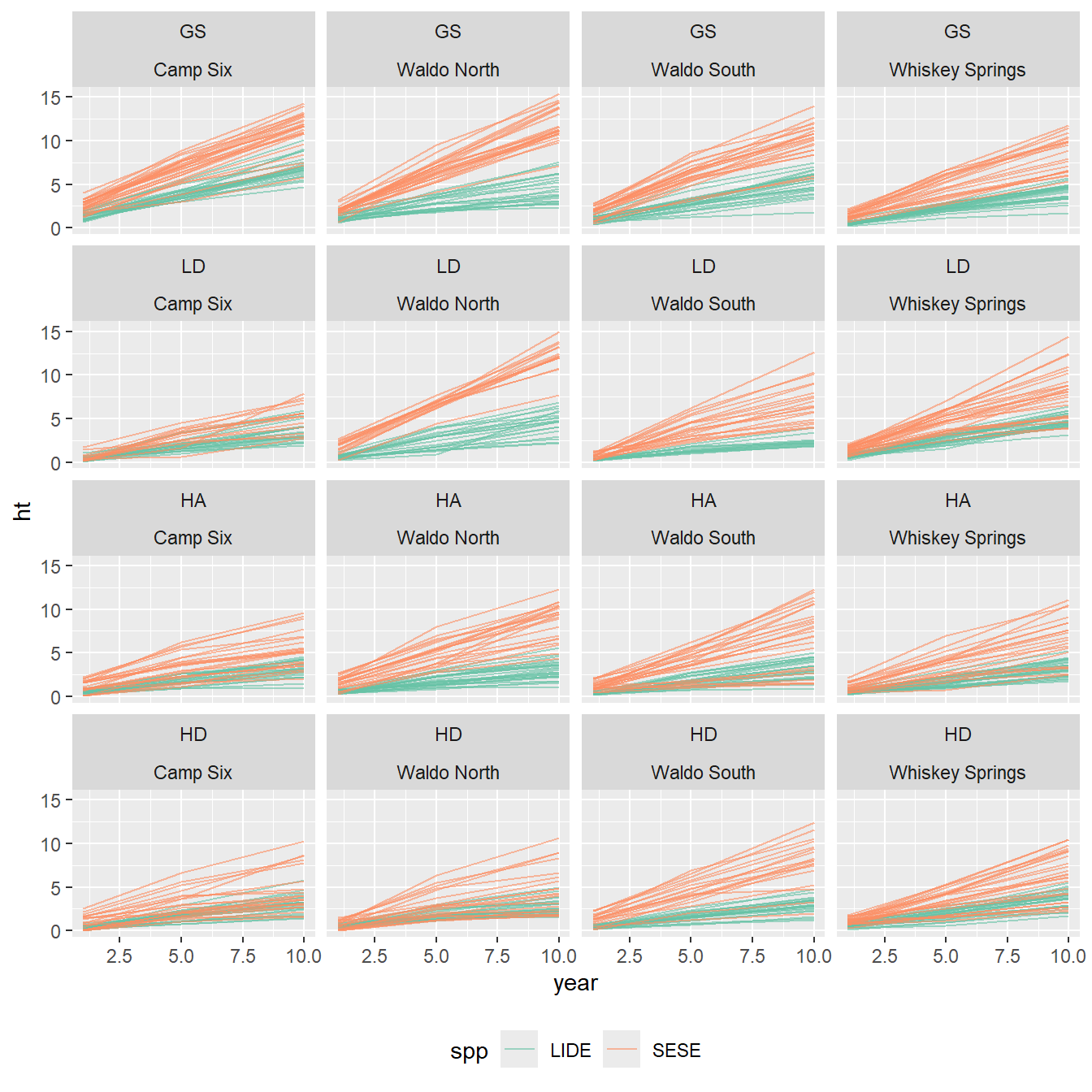
We saw in Figure 8.6 that increment does slow down somewhat in the second measurement period (year 5-10), at least for redwoods, but we may be justified in overlooking this. Lets look at individual tree’s height trajectories.
There are overall treatment effect on growth which varies by species (redwood is more affected) but there are no more significant interactions with year. Our data does not detect significant differences in slow down by treatment or species. j
ht_inc ~ year + spp + treat
This includes only additive effects and the effect of year is the same as model 1.
ht_inc ~ year + spp + treat + spp:treat
Again, the species by treatment interactions seem to be significant.
Adding a random slope for species by plot results in another big jump in AIC, but also reduces confidence in the treatment*species interaction. It would seem that the potential differences in species by treatment growth rate are obscured by redwoods greater variability across plots.
The model selected based on AIC lacks a treatment x species interaction, suggesting that there is not evidence that treatments affected species differentially. It also lacks a treatment x year interaction. This means that there was not enough evidence to support that treatment was related to changes in growth rate.
The presence of treatment in the model (0.001 ≤ p < 0.03) suggests that the levels of treatment were associated with different growth rates across species and years. And the species x year interaction (p < 0.001) suggests changes in growth rates are different for redwood and tanoak.
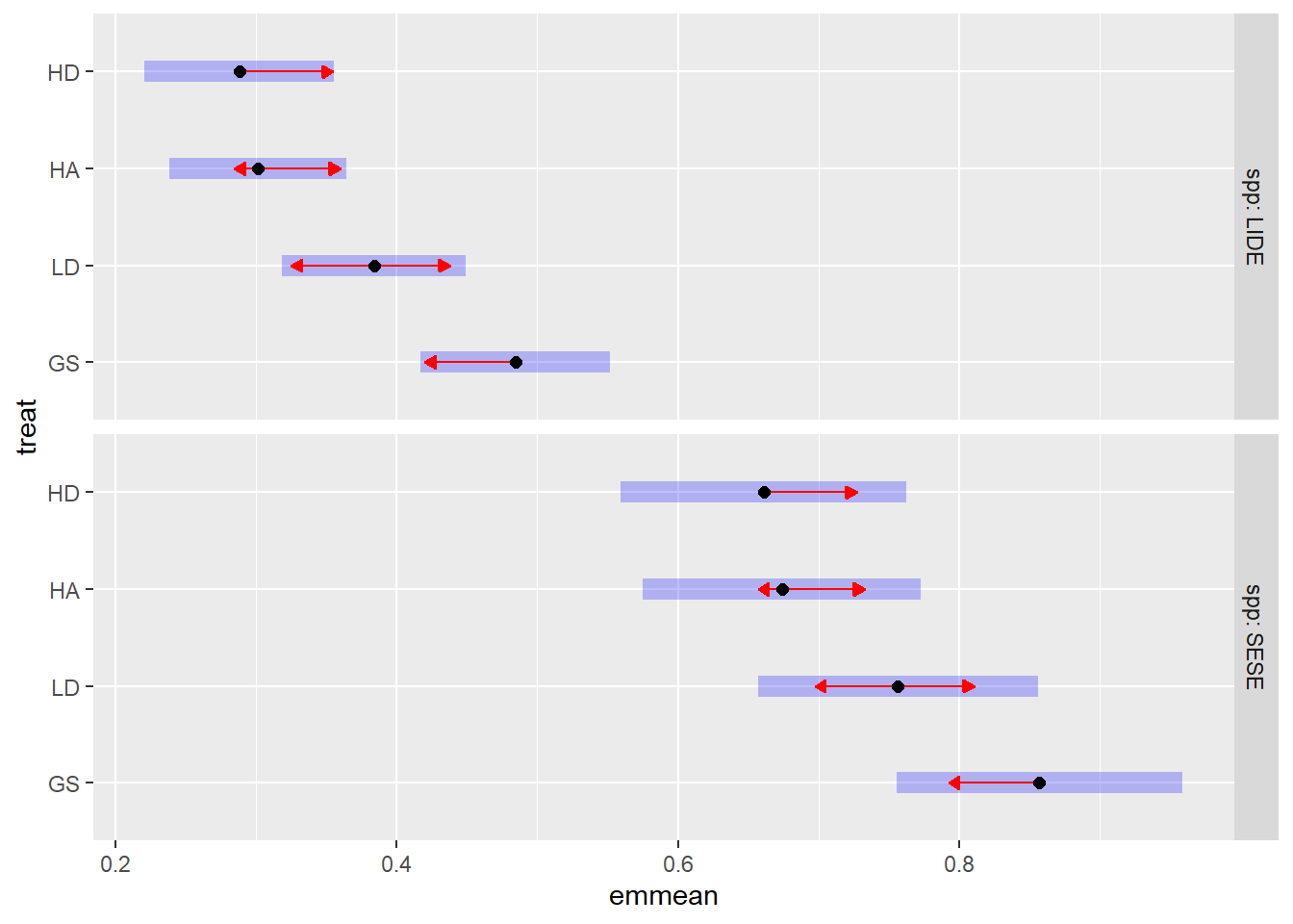
Averaging over growth periods, treatment specific height increments for redwood ranged from 0.66 to 0.86 m yr-1, and for tanoak, from 0.29 to 0.49, with the slowest growth in the HD treatment and the fastest in the GS treatment. height increment was greater in the GS treatment than the HA and HD treatments by about 0.19 m yr-1 (p < 0.001). The LD treatment was intermediate, but not statistically distinguishable from the other treatments (0.13 < p < 0.28).
Code
emm_treat <-emmeans(minc_sel, "treat", by ="spp")plot(emm_treat, comparisons =TRUE)
Figure 9.2: Estimated marginal means for the effect of harvest treatment on redwood and tanoak sprout height increment, averaged over two growth periods, ten years after harvest. Purple bars represent confidence intervals and statistical significance (α = 0.05) is indicated by non-overlaping red arrows.
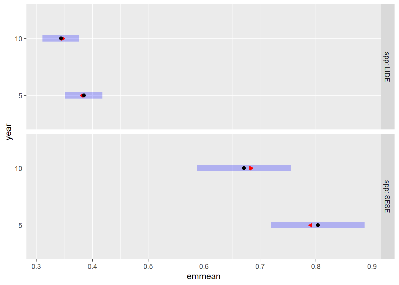
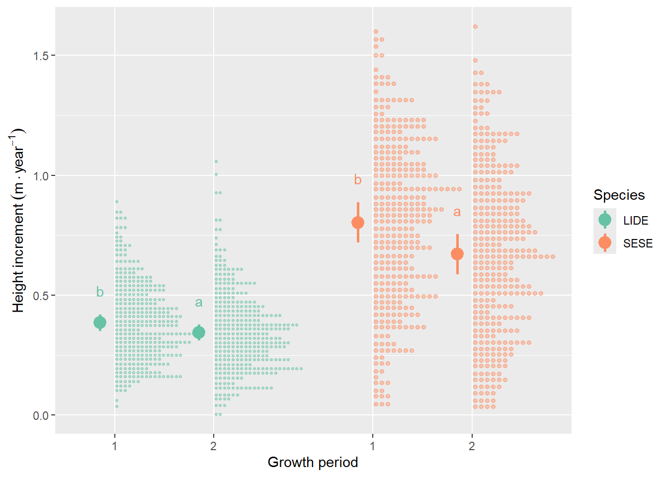
Redwood growth slowed from 0.80 to 0.67 m yr-1 in the second period and tanoak slowed from 0.39 to 0.34 m yr-1.
Redwood grew faster than tanoak, but slowed down more relative to it in the second period. Height increment for redwood was 0.42 m yr-1 greater in the first period and 0.33 m yr-1 greater in the second period than tanoak height increment.
Code
emmeans(minc_sel, c("year"), by ="spp") |>plot(comparisons =TRUE)
Figure 9.3: Estimated marginal means for the effect of growth period on redwood and tanoak sprout height increment, averaged over four harvest treatments, ten years after harvest. Purple bars represent confidence intervals and statistical significance (α = 0.05) is indicated by non-overlaping red arrows.
Code
#| Growth period 1 is year 1-5, growth period 2 is year 5-10. Growth#| significantly decreased in the second period for both species.minc11con |> knitr::kable(digits =3)
Figure 9.4: There was a significant difference in height increment between period 1 and 2 for both species.
9.2.3 Heights - year 10 only
The simplest model that I’m willing to look at includes a treatment/species interaction, and no random effects. It will serve as a baseline for comparison.
# I'm calling the height data "d"dht10 <- sprouts |>lengthen_data("ht") |>filter(year ==10)mht101 <-lm(ht ~ treat * spp, data = dht10)mht102 <-lmer(ht ~ treat * spp + (1| plot) + (1| site), data = dht10)
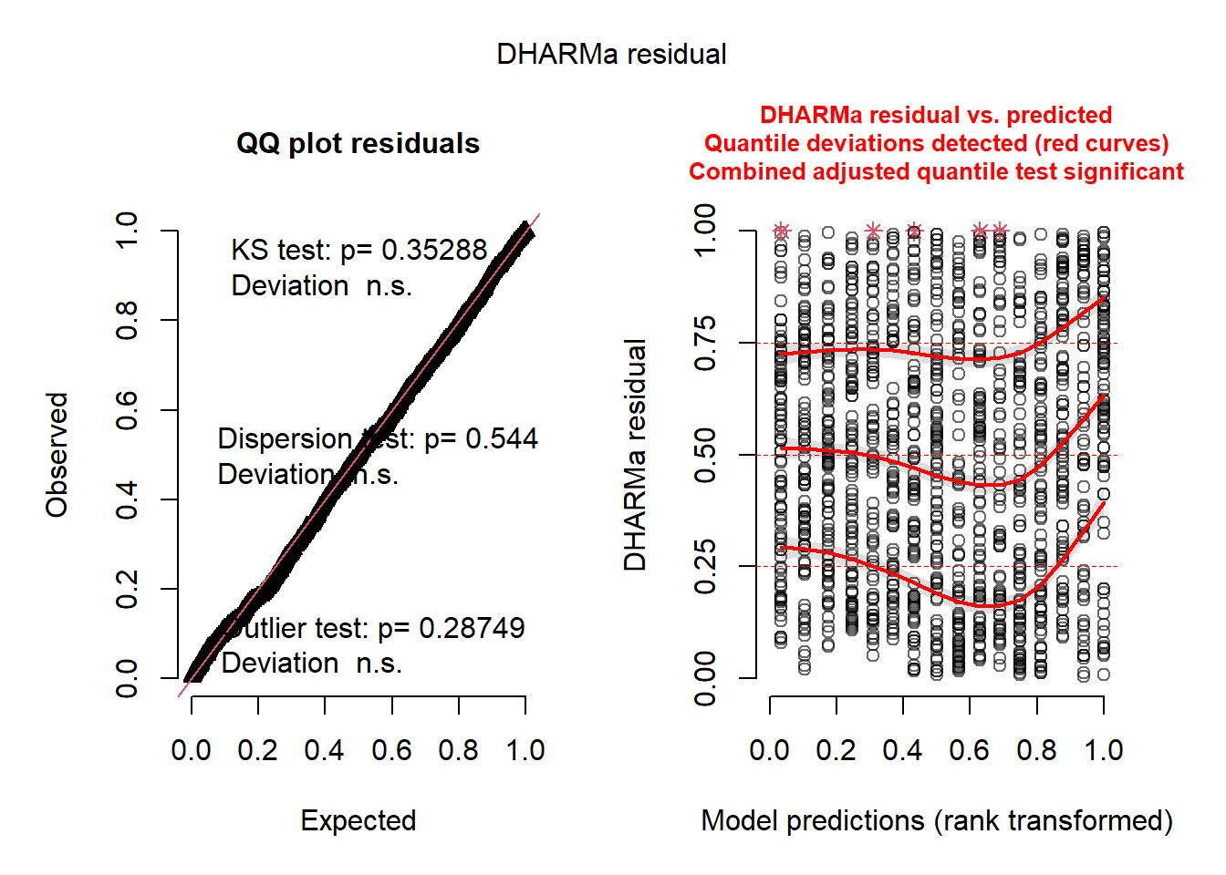
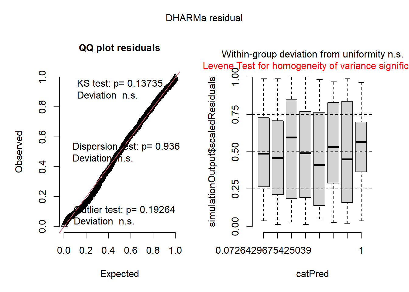
We can see the residuals are not perfect, but nor are they very offensive.
Code
plot(simulateResiduals(mht109))
9.2.4 Here I make my selection
Code
ht10_sel <- mht109
9.2.5 Year 10 only Results
9.2.5.1 Random effects
The best model according to AIC includes a random intercept for plot and a random slope for spp. Because spp is a factor, this effectively estimates a species specific intercept, but also takes into account the covariance of the species plot effect.
9.2.5.2 Fixed effects
The best model included speceis and treatment, but no interactions. This suggests that treatments do not affect species differentially.
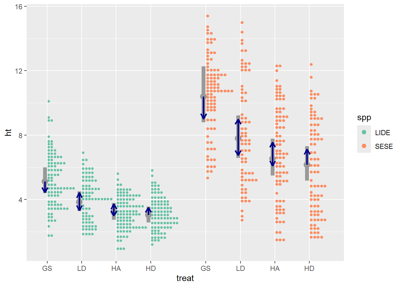
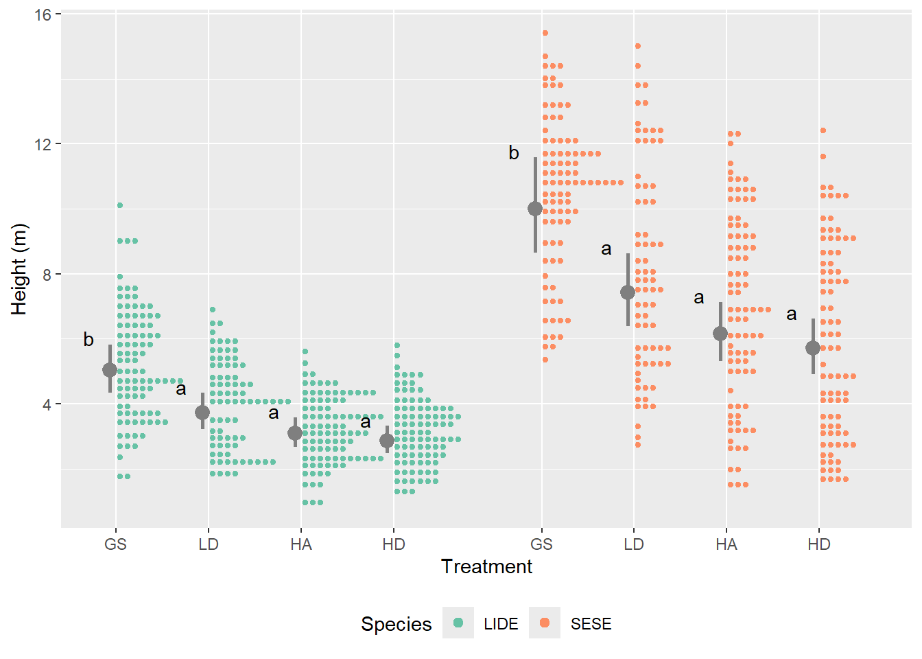
Because the best model did not contain a species x treatment interaction, comparisons between treatments is the same for both species. The GS treatment resulted in greater heights in year 10 than the other treatments (0.001 < p < 0.04). Predicted mean height for redwood ranged from 10.29 m in the GS treatment to 6.16 m in the HD treatment. For tanoak, predicted mean height ranged from 5.12 in the GS treatment to 3.04 in the HD treatment. Predicted mean heights followed the pattern GS > LD > HA > HD.
Warning: Removed 1 row containing missing values or values outside the scale range
(`geom_segment()`).
Removed 1 row containing missing values or values outside the scale range
(`geom_segment()`).
Removed 1 row containing missing values or values outside the scale range
(`geom_segment()`).
Removed 1 row containing missing values or values outside the scale range
(`geom_segment()`).
Figure 9.5: Predicted mean height and 95% confidence intervals (gray bars) for redwood and tanoak stump sprouts 10 years after harvest using four different harvest treatments. Non-overlaping blue arrows indicate statistically significant differences between treatments within a species.
9.2.6 Heights - multiple years
By including year as a numeric variable, we are assuming a liner relationship between year and height. This term (and it’s interactions) can than be interpreted as a modeled growth increment, and although we only have observations at years 1, 5, and 10, other years predictions will be linearly interpolated.
The following models were fit, and are summarized in Table 9.1.
OLS linear model including year in a 3-way interaction.
Eliminate the 3-way interaction (spp:treat:year), keeping others. This results in a significantly lower AIC.
First random-effects model including interactions and universal random slopes for site and plot, and time-series.
Allow the random effects to (co-) vary by species.
Same as 5, but attempt to remove the 3-way interaction again.
Same as 6, but attempt to simplify the random effects by forcing them to be estimated independently, correlation between species is not estimated.
Re-introduce the 3-way interaction again.
Omit the random effect for site. This is supported by the interpretation of
Like 9, but try simplified (independent) random effects.
One problem with this is that I’m comparing AIC for different random effects using ML, when I should be using REML. This may be a problem throughout my model selection.
mht10 <-lmer( ht ~ treat * spp * year + (1| plot:spp) + (1| tree:spp),data = dht)# I tried fitting year as a factor, but then could not fit a model that included# the 3-way interaction and random slopes for species. The model without the# 3-way (and spp random slopes) was close, but about 12 AIC larger.modelsummary(list("Model 2"= mht2,"Model 3"= mht3,"Model 4"= mht4,"Model 5"= mht5,"Model 6"= mht6,"Model 7"= mht7,"Model 8"= mht8,"Model 9"= mht9,"Model 10"= mht10 ),stars =TRUE,output ="markdown",metrics =c("AIC", "BIC", "RMSE"),estimator ="ML",gof_omit ="F|Log.Lik")
Table 9.1: Summary table for models 2-10, described above. Standard error in parantheses.
Model 2
Model 3
Model 4
Model 5
Model 6
Model 7
Model 8
Model 9
Model 10
+ p < 0.1, * p < 0.05, ** p < 0.01, *** p < 0.001
(Intercept)
0.552***
0.232+
0.559
0.546*
0.226
0.226
0.546
0.546*
0.546
(0.156)
(0.136)
(0.350)
(0.261)
(0.255)
(0.425)
(0.428)
(0.260)
(0.428)
treatLD
-0.369
-0.120
-0.421
-0.441
-0.191
-0.193
-0.442
-0.441
-0.442
(0.230)
(0.190)
(0.499)
(0.364)
(0.361)
(0.593)
(0.599)
(0.371)
(0.609)
treatHA
-0.372+
0.035
-0.390
-0.367
0.040
0.041
-0.366
-0.367
-0.366
(0.219)
(0.180)
(0.495)
(0.361)
(0.358)
(0.589)
(0.595)
(0.368)
(0.605)
treatHD
-0.348
0.258
-0.350
-0.345
0.262
0.262
-0.345
-0.345
-0.345
(0.220)
(0.181)
(0.495)
(0.361)
(0.358)
(0.589)
(0.596)
(0.368)
(0.605)
sppSESE
0.572**
1.215***
0.527*
0.535
1.178*
1.182*
0.539
0.535
0.539
(0.221)
(0.158)
(0.205)
(0.473)
(0.474)
(0.596)
(0.606)
(0.474)
(0.606)
year
0.471***
0.531***
0.471***
0.471***
0.531***
0.531***
0.471***
0.471***
0.471***
(0.024)
(0.019)
(0.017)
(0.017)
(0.013)
(0.013)
(0.017)
(0.017)
(0.017)
treatLD × sppSESE
-0.311
-0.807***
-0.224
-0.181
-0.677
-0.669
-0.173
-0.175
-0.173
(0.330)
(0.188)
(0.307)
(0.533)
(0.500)
(0.828)
(0.849)
(0.679)
(0.862)
treatHA × sppSESE
-0.100
-0.925***
-0.039
-0.057
-0.882+
-0.885
-0.060
-0.055
-0.059
(0.314)
(0.179)
(0.291)
(0.524)
(0.493)
(0.824)
(0.843)
(0.672)
(0.857)
treatHD × sppSESE
-0.245
-1.492***
-0.204
-0.186
-1.432**
-1.434+
-0.187
-0.186
-0.187
(0.316)
(0.180)
(0.293)
(0.525)
(0.494)
(0.825)
(0.844)
(0.673)
(0.857)
treatLD × year
-0.085*
-0.132***
-0.085***
-0.085***
-0.132***
-0.132***
-0.085***
-0.085***
-0.085***
(0.036)
(0.026)
(0.025)
(0.025)
(0.018)
(0.018)
(0.025)
(0.025)
(0.025)
treatHA × year
-0.169***
-0.245***
-0.169***
-0.169***
-0.245***
-0.245***
-0.169***
-0.169***
-0.169***
(0.034)
(0.024)
(0.023)
(0.023)
(0.017)
(0.017)
(0.023)
(0.023)
(0.023)
treatHD × year
-0.175***
-0.288***
-0.175***
-0.175***
-0.288***
-0.288***
-0.175***
-0.175***
-0.175***
(0.034)
(0.024)
(0.023)
(0.023)
(0.017)
(0.017)
(0.023)
(0.023)
(0.023)
sppSESE × year
0.481***
0.360***
0.481***
0.481***
0.360***
0.360***
0.481***
0.481***
0.481***
(0.034)
(0.018)
(0.024)
(0.024)
(0.012)
(0.012)
(0.024)
(0.024)
(0.024)
treatLD × sppSESE × year
-0.093+
-0.093**
-0.093**
-0.093**
-0.093**
-0.093**
(0.051)
(0.035)
(0.035)
(0.035)
(0.035)
(0.035)
treatHA × sppSESE × year
-0.155**
-0.155***
-0.155***
-0.155***
-0.155***
-0.155***
(0.048)
(0.033)
(0.033)
(0.033)
(0.033)
(0.033)
treatHD × sppSESE × year
-0.234***
-0.234***
-0.234***
-0.234***
-0.234***
-0.234***
(0.049)
(0.034)
(0.034)
(0.034)
(0.034)
(0.034)
SD (Observations)
1.016
1.016
1.031
1.034
1.016
1.016
1.016
SD (Intercept treespp)
0.844
0.852
0.852
SD (Intercept plotspp)
0.795
0.795
0.809
SD (Intercept site)
0.000
SD (sppLIDE site)
0.103
0.000
SD (sppSESE site)
0.488
0.629
Cor (sppLIDE~sppSESE site)
-1.000
SD (Intercept sitespp)
0.153
0.153
SD (Intercept tree)
0.925
SD (sppLIDE tree)
0.004
0.000
0.000
SD (sppSESE tree)
1.227
1.223
1.227
Cor (sppLIDE~sppSESE tree)
-0.103
0.450
0.284
SD (Intercept plot)
0.638
SD (sppLIDE plot)
0.463
0.474
0.474
SD (sppSESE plot)
0.914
0.919
1.037
Cor (sppLIDE~sppSESE plot)
0.783
0.782
0.570
Num.Obs.
2076
2076
2076
2076
2076
2076
2076
2076
2076
AIC
7518.3
7536.9
6890.7
6631.3
6677.1
6896.9
6851.9
6629.7
6849.9
BIC
7614.1
7615.9
7003.5
6777.9
6806.8
6992.7
6964.7
6759.4
6957.1
RMSE
1.47
1.48
0.88
0.94
0.96
0.91
0.89
0.94
0.89
9.2.7 Multi-year heights V2
The problem with all of the above models is (a) a normal distribution is not a good fit for the data because it results in negative height predictions for small trees (year 1) and (b) variance is not constant. Finally, we are fitting year as a linear effect because fitting it as a factor with 3 levels led to model convergence problems, but ideally, we would like to allow different relationships between height and year, because, as we saw in the previous section, height growth is not constant in the first 10 years.
For these reasons it makes sense to try another modeling framework, particularly, a gamma distributed model, with a modeled dispersion parameter. It allows only positive predictions, can right skewed distributions, and the dispersion can be modeled as a function of covariates.
Table 9.2: Summary table for models 2-10, described above. Standard error in parantheses.
Model 11
Model 12
Model 13
Model 14
Model 15
Model 16
Model 17
Model 18
+ p < 0.1, * p < 0.05, ** p < 0.01, *** p < 0.001
(Intercept) conditional
-0.096
-0.118
-0.114
-0.104
-0.101
-0.095
-0.101
-0.107
(0.101)
(0.098)
(0.101)
(0.090)
(0.089)
(0.085)
(0.079)
treatLD conditional
-0.608***
-0.612***
-0.625
-0.663***
-0.628***
-0.628***
-0.614***
-0.616***
(0.145)
(0.138)
(0.143)
(0.126)
(0.126)
(0.124)
(0.112)
treatHA conditional
-0.723***
-0.659***
-0.655
-0.675***
-0.621***
-0.643***
-0.629***
-0.665***
(0.142)
(0.136)
(0.141)
(0.124)
(0.124)
(0.121)
(0.110)
treatHD conditional
-0.679***
-0.656***
-0.660
-0.696***
-0.669***
-0.675***
-0.663***
-0.740***
(0.143)
(0.137)
(0.141)
(0.124)
(0.124)
(0.121)
(0.110)
sppSESE conditional
0.710***
0.754***
0.751
0.739***
0.763***
0.766***
0.742***
0.762***
(0.076)
(0.058)
(0.056)
(0.065)
(0.065)
(0.062)
(0.038)
year conditional
0.186***
0.190***
0.190
(0.008)
(0.006)
treatLD × sppSESE conditional
-0.007
0.002
0.014
-0.008
0.000
0.000
0.003
(0.115)
(0.075)
(0.078)
(0.079)
(0.079)
(0.078)
treatHA × sppSESE conditional
0.232*
0.103
0.082
0.100
0.026
0.026
0.028
(0.108)
(0.071)
(0.074)
(0.075)
(0.074)
(0.073)
treatHD × sppSESE conditional
-0.053
-0.100
-0.116
-0.126+
-0.134+
-0.134+
-0.129+
(0.110)
(0.071)
(0.074)
(0.075)
(0.075)
(0.074)
treatLD × year conditional
0.036**
0.037***
0.037
(0.011)
(0.008)
treatHA × year conditional
0.027*
0.015+
0.016
(0.011)
(0.008)
treatHD × year conditional
0.020+
0.016*
0.017
(0.011)
(0.008)
sppSESE × year conditional
0.000
-0.008
-0.008
(0.011)
(0.006)
treatLD × sppSESE × year conditional
0.002
(0.016)
treatHA × sppSESE × year conditional
-0.024
(0.015)
treatHD × sppSESE × year conditional
-0.009
(0.016)
(Intercept) dispersion
0.430
0.431
0.429
0.330
1.370***
1.599***
1.950***
-1.147***
(0.053)
(0.075)
(0.114)
(0.055)
year5 conditional
1.176***
1.147***
1.142***
1.147***
1.158***
(0.039)
(0.043)
(0.041)
(0.033)
(0.028)
year10 conditional
1.748***
1.720***
1.714***
1.719***
1.721***
(0.039)
(0.044)
(0.041)
(0.034)
(0.030)
treatLD × year5 conditional
0.326***
0.286***
0.286***
0.275***
0.279***
(0.052)
(0.057)
(0.056)
(0.053)
(0.042)
treatHA × year5 conditional
0.110*
0.081
0.103+
0.091+
0.155***
(0.049)
(0.054)
(0.053)
(0.047)
(0.038)
treatHD × year5 conditional
0.168***
0.138*
0.144**
0.132**
0.158***
(0.050)
(0.055)
(0.054)
(0.049)
(0.038)
treatLD × year10 conditional
0.367***
0.330***
0.329***
0.315***
0.318***
(0.052)
(0.058)
(0.057)
(0.054)
(0.044)
treatHA × year10 conditional
0.141**
0.110*
0.133*
0.117*
0.178***
(0.049)
(0.055)
(0.054)
(0.048)
(0.040)
treatHD × year10 conditional
0.172***
0.143*
0.149**
0.137**
0.178***
(0.050)
(0.056)
(0.055)
(0.050)
(0.040)
sppSESE × year5 conditional
-0.028
-0.031
-0.035
-0.016
-0.049+
(0.036)
(0.039)
(0.040)
(0.036)
(0.029)
sppSESE × year10 conditional
-0.062+
-0.069+
-0.071+
-0.043
-0.073*
(0.036)
(0.040)
(0.041)
(0.037)
(0.030)
year5 dispersion
2.957***
2.650***
2.716***
-0.339**
(0.146)
(0.193)
(0.202)
(0.115)
year10 dispersion
2.409***
2.200***
2.188***
0.863***
(0.116)
(0.164)
(0.160)
(0.050)
sppSESE dispersion
-0.422***
0.610***
0.301***
(0.107)
(0.166)
(0.074)
year5 × sppSESE dispersion
0.568*
0.460
(0.286)
(0.297)
year10 × sppSESE dispersion
0.389+
0.291
(0.231)
(0.225)
treatLD dispersion
-0.571***
-0.169*
(0.151)
(0.077)
treatHA dispersion
-0.441**
-0.434***
(0.144)
(0.074)
treatHD dispersion
-0.379**
-0.411***
(0.145)
(0.074)
sppSESE × treatLD dispersion
-1.054***
0.299**
(0.216)
(0.110)
sppSESE × treatHA dispersion
-1.024***
0.546***
(0.208)
(0.108)
sppSESE × treatHD dispersion
-1.312***
0.424***
(0.211)
(0.108)
SD (Intercept tree) conditional
0.225
0.225
0.294
0.344
0.344
0.341
0.330
SD (sppLIDE tree) conditional
0.101
SD (sppSESE tree) conditional
0.291
Cor (sppLIDE~sppSESE tree) conditional
0.000
SD (Intercept plot) conditional
0.170
0.170
0.182
0.141
0.141
0.141
0.138
SD (sppLIDE plot) conditional
0.180
SD (sppSESE plot) conditional
0.214
Cor (sppLIDE~sppSESE plot) conditional
0.637
Num.Obs.
2076
2076
2076
2076
2076
2076
2076
2076
AIC
6173.1
6170.5
6119.9
5448.4
4544.8
4534.7
4398.6
4278.4
BIC
6280.2
6260.7
6232.6
5566.8
4674.5
4681.3
4579.0
4430.6
RMSE
1.16
1.15
1.12
0.73
0.45
0.45
0.46
0.50
The model with the lowest AIC is model 18.
9.2.8 Multi-year model checking
Code
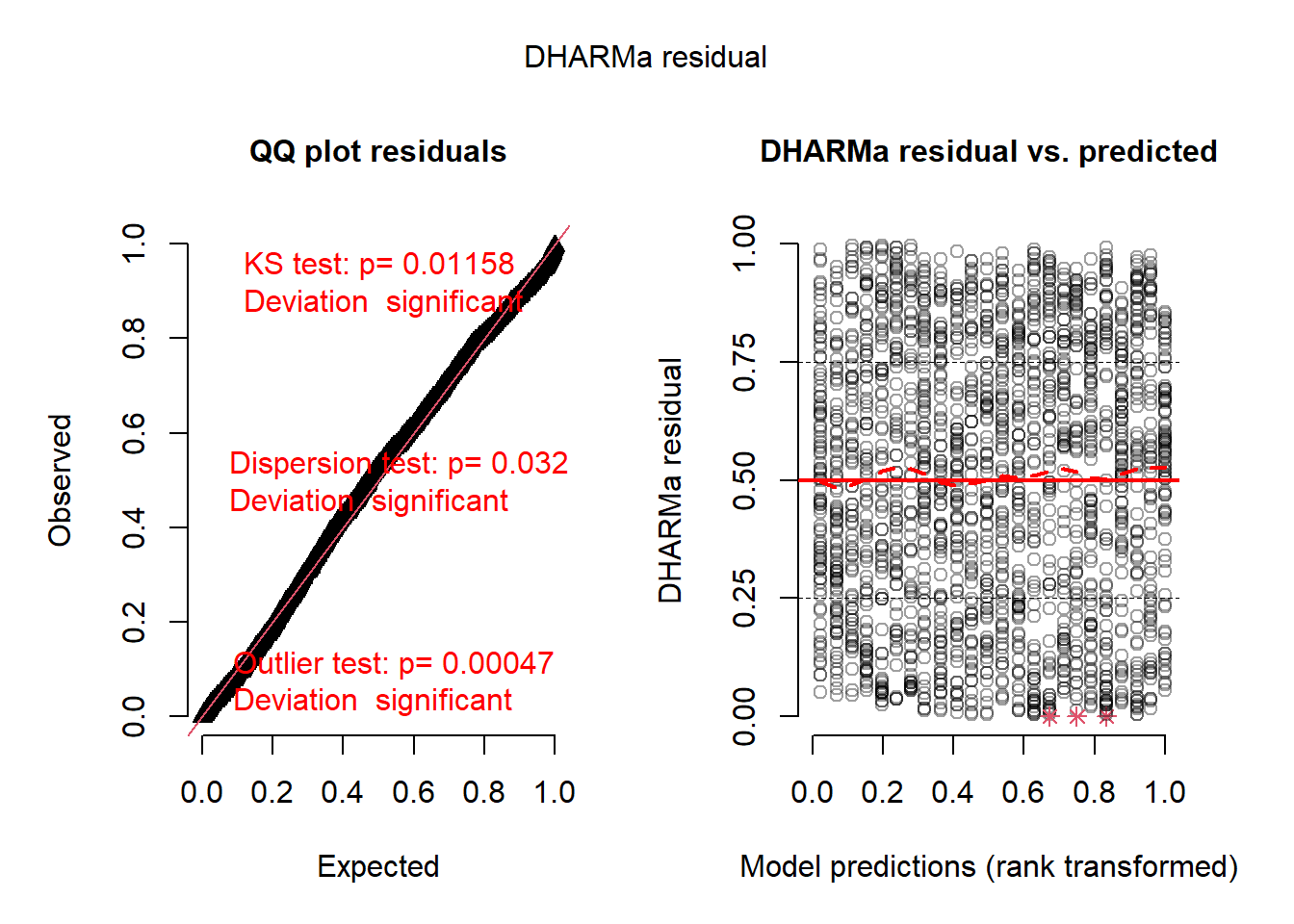
res <-simulateResiduals(mht18)plot(res)
Figure 9.6: Residual vs fitted plot for the selected multi-year linear regression model for heights.
9.2.9 Multi-year results
Using model 18, we can now answer the questions we posed in the Objectives section.
Code
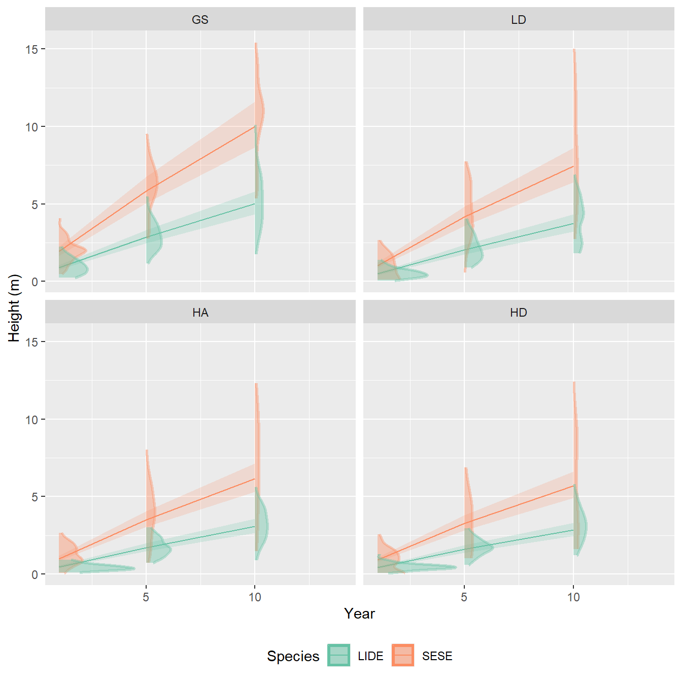
mht18emmeans <-emmeans( mht18,c("spp", "treat", "year"),type ="response")mht18emmeans |>as_tibble() |>mutate(year =as.numeric(levels(year))[year] ) |>rename(any_of(c(lower.CL ="asymp.LCL", upper.CL ="asymp.UCL"))) |>ggplot(aes(year, response, color = spp, fill = spp, group = spp)) +geom_line() +facet_wrap(~treat) +geom_ribbon(aes(ymin = lower.CL, ymax = upper.CL, color =NULL),alpha = .2 ) +stat_slab(data = dht, aes(year, ht), alpha =0.4) +scale_color_brewer(palette ="Set2", aesthetics =c("color", "fill")) +theme(legend.position ="bottom") +labs(x ="Year", y ="Height (m)", color ="Species", fill ="Species")
Figure 9.7: Average species and treatment specific height as a linear function of year. Density distributions represent the raw data associated with the estimate at that point. The grey line is the OLS fit for reference.
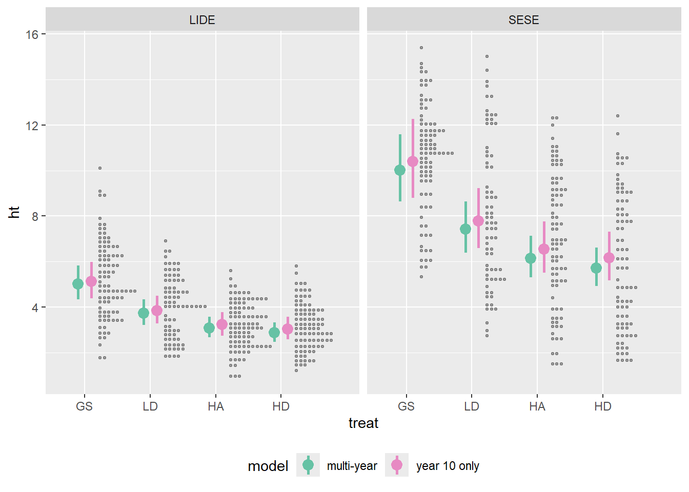
Figure 9.8: Marginal means at year 10 based on height data collected three times over 10 years. The same letter within a species indicates that there was not enough evidence to differentiate those treatments.
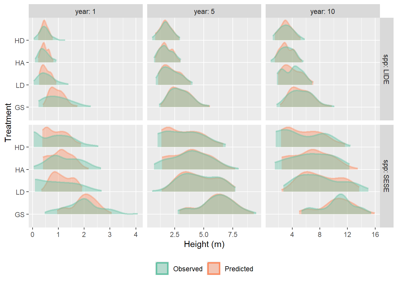
Figure 9.9: Oberved and predicted height distribution of our observed dataset using the final, chosen, multi-year model. Predictions were made using all random effects.
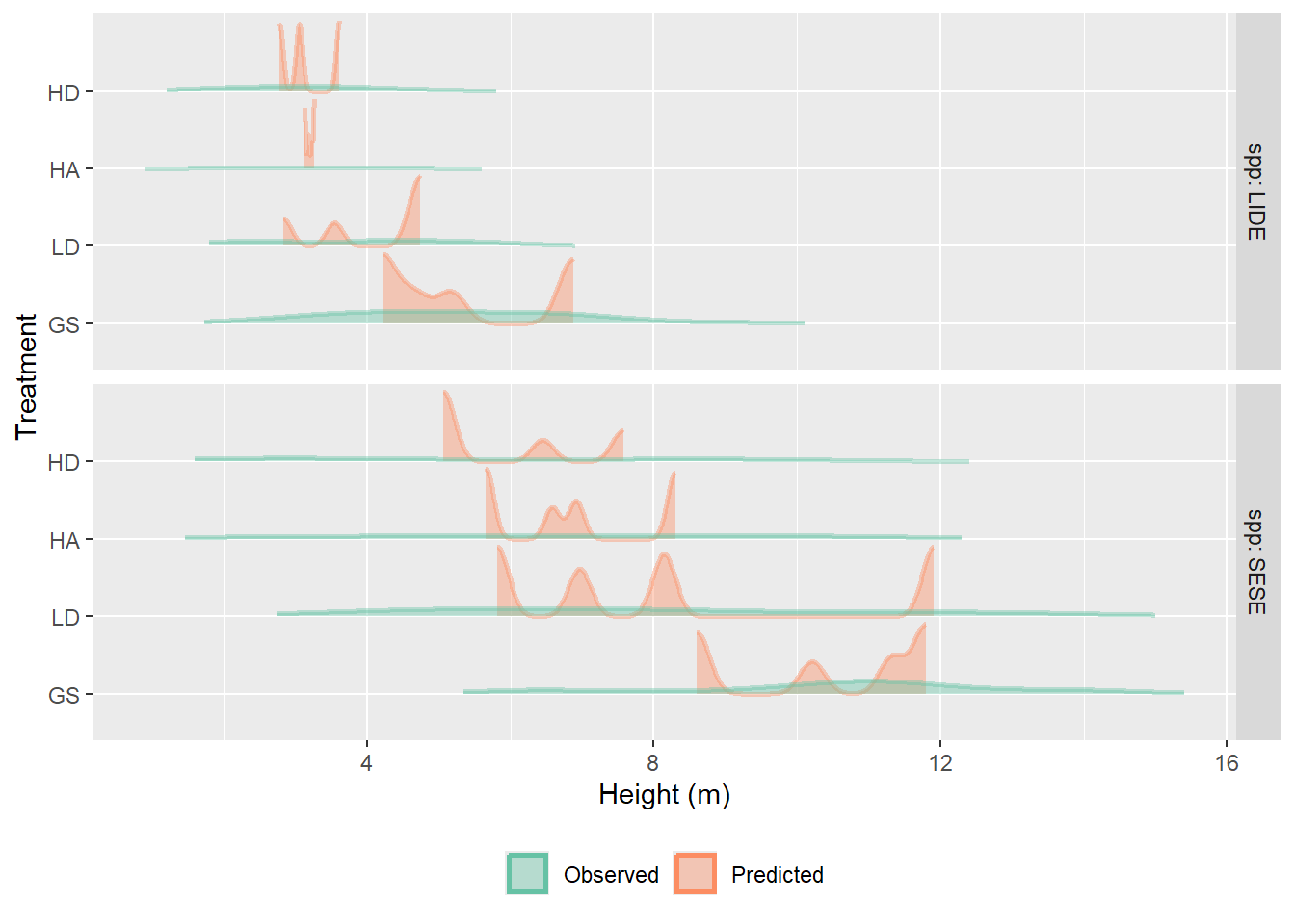
Code
#| label: fig-height-pred-fit-10-only#| fig-cap: >#| Oberved and predicted height distribution of our observed dataset using the#| selected year-10-only model.#| Predictions were made using all random effects.sprouts |>lengthen_data("ht") |>filter(year =="10") |>mutate(Predicted =predict( ht10_sel,lst(site, plot, tree, treat, spp, year),type ="response" ),Observed = ht ) |>pivot_longer(c(Observed, Predicted)) |>ggplot(aes(value, treat, color = name, fill = name)) +stat_slab(alpha =0.4, normalize ="xy") +facet_grid(vars(spp), scales ="free", labeller = label_both) +labs(x ="Height (m)", y ="Treatment") +scale_color_brewer(palette ="Set2", aesthetics =c("color", "fill")) +theme(legend.position ="bottom", legend.title =element_blank())