bf3 <- mutate(
d,
priors = list(brms::set_prior(
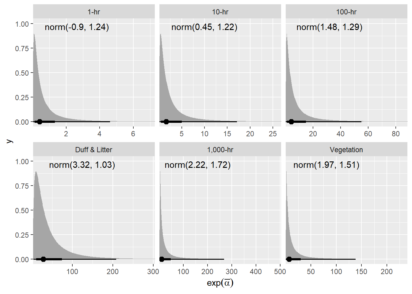
str_glue("normal({mu}, {sigma})", .envir = lnp(data$load))
)),
mod = list(brms::brm(
form,
data,
warmup = 5000,
iter = 6000,
cores = 4,
control = list(adapt_delta = 0.99),
family = brms::hurdle_gamma(),
prior = priors,
file = paste0("fits/bf3_", class)
))
)
bf4 <- mutate(
d,
priors = list(
set_prior(
str_glue("normal({mu}, {sigma})", .envir = lnp(data$load)),
nlpar = "a",
coef = "Intercept"
) +
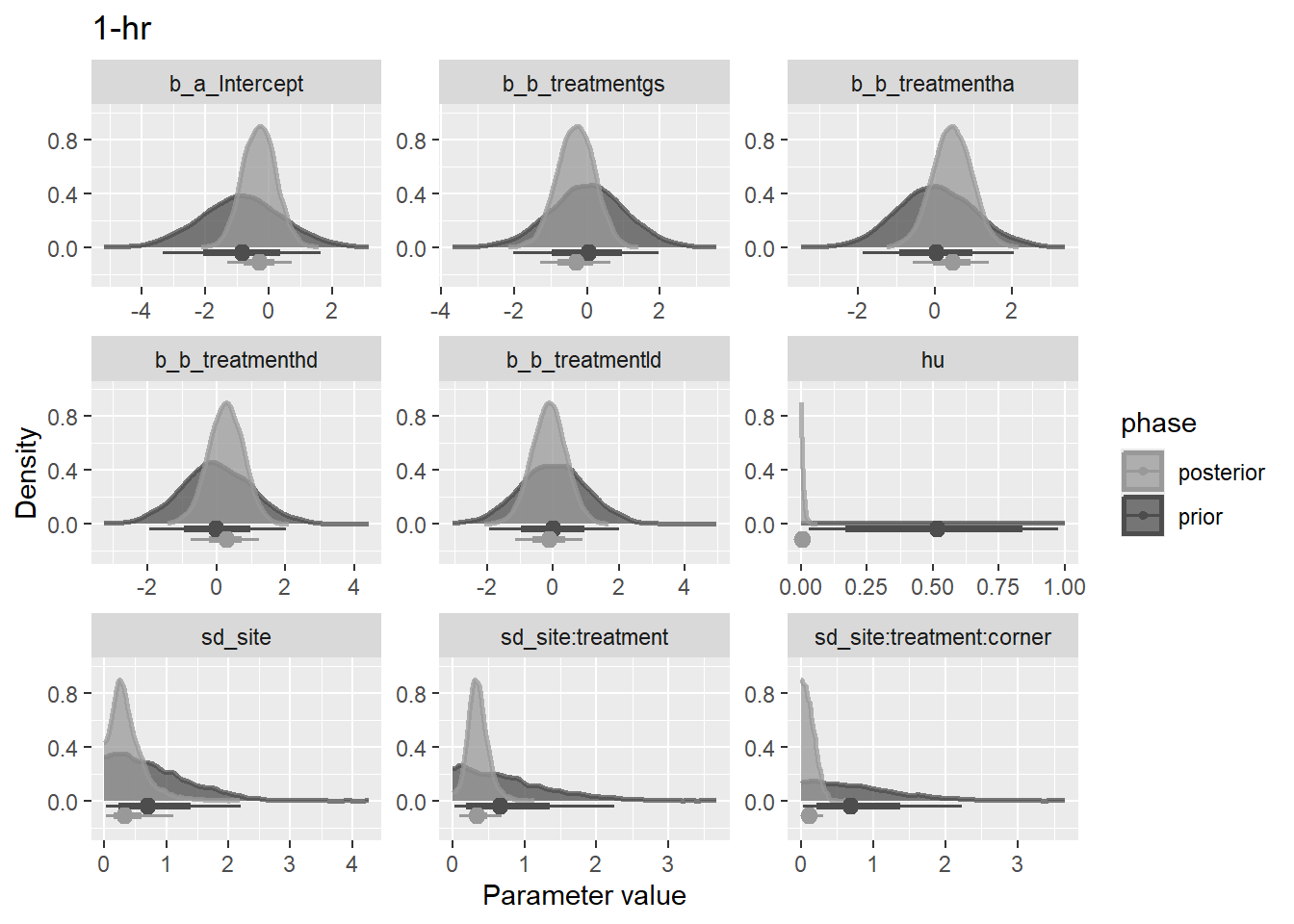
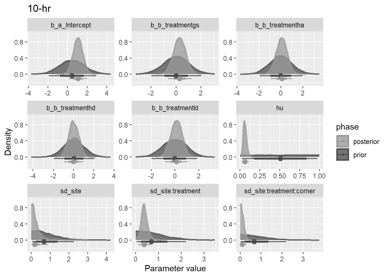
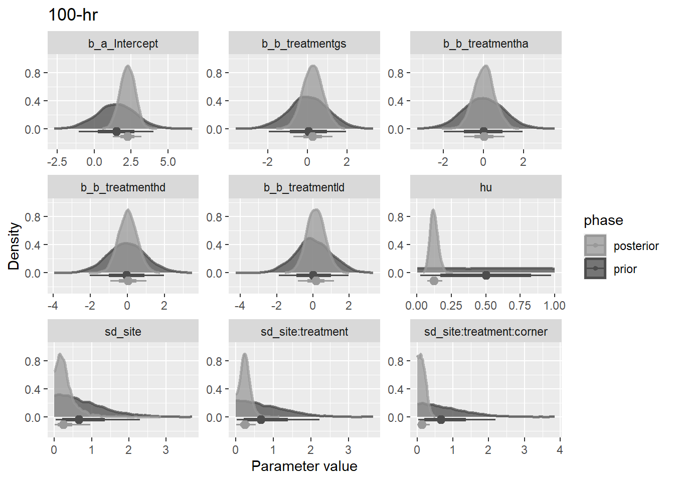
set_prior("student_t(3, 0, 0.35)", nlpar = "a", class = "sd") +
set_prior("student_t(3, 0, 0.35)", nlpar = "b", coef = "treatmentgs") +
set_prior("student_t(3, 0, 0.35)", nlpar = "b", coef = "treatmentha") +
set_prior("student_t(3, 0, 0.35)", nlpar = "b", coef = "treatmenthd") +
set_prior("student_t(3, 0, 0.35)", nlpar = "b", coef = "treatmentld")
),
mod = list(brms::brm(
brms::bf(
load ~ a + b,
a ~ 1 + (1 | site / treatment / corner),
b ~ 0 + treatment,
nl = TRUE
),
data,
warmup = 4000,
iter = 5000,
cores = 4,
control = list(adapt_delta = 0.99),
family = brms::hurdle_gamma(),
prior = priors,
sample_prior = TRUE,
file = paste0("fits/bf4_", class)
))
)
bf5 <- mutate(
d,
priors = list(brms::set_prior(
str_glue("normal({mu}, {sigma})", .envir = lnp(data$load))
)),
mod = list(brms::brm(
brms::bf(
load ~ 0 + Intercept + (1 | site / treatment / corner) + (1 | treatment)
),
data,
warmup = 4000,
iter = 5000,
cores = 4,
control = list(adapt_delta = 0.99),
family = brms::hurdle_gamma(),
prior = priors,
file = paste0("fits/bf5_", class)
))
)